- Some wow graphics to show you up front what R can do to help you visualize the patterns in your data:
> demo()

> demo(package = .packages(all.available = TRUE))
>
>
> demo(graphics)


        demo(graphics)
        ---- ~~~~~~~~

Type     to start :
- ls() lists the contents of your workspace.
> ls()
 [1] "b"            "bmi"          "bp.obese"     "c"            "caesar.shoe"
 [6] "coking"       "d"            "daily.intake" "energy"       "fake.trypsin"
[11] "heart.rate"   "hh"           "ht"           "ht2"          "IgM"
[16] "intake"       "juul"         "LETTERS"      "m"            "wt"
[21] "x"            "xbar"
- Using sequences, concatenate, etc.
> myVector<-c(11,22.2,33,44,55,66)

> myVector2 <- c(1.3, 1.4, 1.6, 1.75, 1.9, 2.1)

> seq(1,40,2)
 [1]  1  3  5  7  9 11 13 15 17 19 21 23 25 27 29 31 33 35 37 39

> c<-seq(11,30,2)
> c
 [1] 11 13 15 17 19 21 23 25 27 29

> d<-seq(1,20)
> d
 [1]  1  2  3  4  5  6  7  8  9 10 11 12 13 14 15 16 17 18 19 20

> d*2-1
 [1]  1  3  5  7  9 11 13 15 17 19 21 23 25 27 29 31 33 35 37 39

> letters
 [1] "a" "b" "c" "d" "e" "f" "g" "h" "i" "j" "k" "l" "m" "n" "o" "p" "q" "r" "s" "t" "u" "v"
[23] "w" "x" "y" "z"
- Postional arguments and named argument. pch is the NAME of an argument. Postional matching is used on 1st plot, both positional and named actual argument approach is used on the 2nd plot, and finally the 3rd plot uses only named actual arguments.
>
> plot(myVector,myVector2)
>
> plot(myVector,myVector2,pch=8)

> plot(pch=3,y=myVector2,x=myVector)
- Pages 83-84 of Peter Dalgaard Introductory Statistics with R - daily energy intake in kJ for 11 women.
> daily.intake <- c(5260,5470,5640,6180,6390,6515,6805,7515,7515,8230,8770)

> mean(daily.intake)
[1] 6753.636

> sd(daily.intake)
[1] 1142.123

> quantile(daily.intake)
  0%  25%  50%  75% 100%
5260 5910 6515 7515 8770

> t.test(daily.intake,mu=7725)

        One Sample t-test

data:  daily.intake
t = -2.8208, df = 10, p-value = 0.01814
alternative hypothesis: true mean is not equal to 7725
95 percent confidence interval:
 5986.348 7520.925
sample estimates:
mean of x
 6753.636
- How do you get the data frames that are used in many of the R tutorials and that are used in the Peter Dalgaard book for all examples?
> library(ISwR)

                energy, intake and juul are three of the many data sets in the ISwR library.
                ------  ------     ----
- Two-sample t test - daily energy expenditure comparisons - lean versus obese women study.
> data(energy)
> attach(energy)
> energy
   expend stature
1    9.21   obese
2    7.53    lean
3    7.48    lean
4    8.08    lean
5    8.09    lean
6   10.15    lean
7    8.40    lean
8   10.88    lean
9    6.13    lean
10   7.90    lean
11  11.51   obese
12  12.79   obese
13   7.05    lean
14  11.85   obese
15   9.97   obese
16   7.48    lean
17   8.79   obese
18   9.69   obese
19   9.68   obese
20   7.58    lean
21   9.19   obese
22   8.11    lean

> t.test(expend~stature)

        Welch Two Sample t-test

data:  expend by stature
t = -3.8555, df = 15.919, p-value = 0.001411
alternative hypothesis: true difference in means is not equal to 0
95 percent confidence interval:
 -3.459167 -1.004081
sample estimates:
 mean in group lean mean in group obese
           8.066154           10.297778

> t.test(expend~stature, var.equal=T)

        Two Sample t-test

data:  expend by stature
t = -3.9456, df = 20, p-value = 0.000799
alternative hypothesis: true difference in means is not equal to 0
95 percent confidence interval:
 -3.411451 -1.051796
sample estimates:
 mean in group lean mean in group obese
           8.066154           10.297778
- Are the group variances the same? Using the var.test R function to test the equal variances assumption. Section 4.4 of Dalgaard book. Comparison of variances.
> var.test(expend~stature)

        F test to compare two variances

data:  expend by stature
F = 0.7844, num df = 12, denom df = 8, p-value = 0.6797
alternative hypothesis: true ratio of variances is not equal to 1
95 percent confidence interval:
 0.1867876 2.7547991
sample estimates:
ratio of variances
          0.784446
- The paired t test examples.
> data(intake)
> attach(intake)
> intake
    pre post
1  5260 3910
2  5470 4220
3  5640 3885
4  6180 5160
5  6390 5645
6  6515 4680
7  6805 5265
8  7515 5975
9  7515 6790
10 8230 6900
11 8770 7335

> post - pre
 [1] -1350 -1250 -1755 -1020  -745 -1835 -1540 -1540  -725 -1330 -1435

 > t.test(pre, post, paired=T)

        Paired t-test

data:  pre and post
t = 11.9414, df = 10, p-value = 3.059e-07
alternative hypothesis: true difference in means is not equal to 0
95 percent confidence interval:
 1074.072 1566.838
sample estimates:
mean of the differences
               1320.455

> t.test(pre, post)  # This is WRONG for above data!!!!

        Welch Two Sample t-test

data:  pre and post
t = 2.6242, df = 19.92, p-value = 0.01629
alternative hypothesis: true difference in means is not equal to 0
95 percent confidence interval:
  270.5633 2370.3458
sample estimates:
mean of x mean of y
 6753.636  5433.182
- The juul data frame has 1,339 rows and 6 columns. IGF1 is Insulin-like Growth Factor. It is measured in mg/l, micrograms per liter.
> data(juul)

> attach(juul)

> mean(igf1)
[1] NA

> mean(igf1,na.rm=T)
[1] 340.168

> summary(igf1)
   Min. 1st Qu.  Median    Mean 3rd Qu.    Max.    NA's
   25.0   202.2   313.5   340.2   462.8   915.0   321.0
- In R, the data sets NA's could be counted like this too, since TRUE is converted to 1 and FALSE is converted to 0 when we apply arithmetic operations or R functions that expect numeric input to TRUE and FALSE.
> sum(!is.na(igf1))
[1] 1018

> sum(is.na(igf1))
[1] 321

> 1018 + 321
[1] 1339         The juul data set is 1,339 rows and 6 columns...
- Making a variable categorical or a factor in R is often necessary.
> summary(juul)
      age            menarche            sex             igf1
 Min.   : 0.170   Min.   :  1.000   Min.   :1.000   Min.   : 25.0
 1st Qu.: 9.053   1st Qu.:  1.000   1st Qu.:1.000   1st Qu.:202.2
 Median :12.560   Median :  1.000   Median :2.000   Median :313.5
 Mean   :15.095   Mean   :  1.476   Mean   :1.534   Mean   :340.2
 3rd Qu.:16.855   3rd Qu.:  2.000   3rd Qu.:2.000   3rd Qu.:462.8
 Max.   :83.000   Max.   :  2.000   Max.   :2.000   Max.   :915.0
 NA's   : 5.000   NA's   :635.000   NA's   :5.000   NA's   :321.0
     tanner           testvol
 Min.   :  1.000   Min.   :  1.000
 1st Qu.:  1.000   1st Qu.:  1.000
 Median :  2.000   Median :  3.000
 Mean   :  2.640   Mean   :  7.896
 3rd Qu.:  5.000   3rd Qu.: 15.000
 Max.   :  5.000   Max.   : 30.000
 NA's   :240.000   NA's   :859.000

> juul$sex <- factor(juul$sex, labels=c("Male","Female"))

> summary(juul)
      age            menarche           sex           igf1
 Min.   : 0.170   Min.   :  1.000   Male  :621   Min.   : 25.0
 1st Qu.: 9.053   1st Qu.:  1.000   Female:713   1st Qu.:202.2
 Median :12.560   Median :  1.000   NA's  :  5   Median :313.5
 Mean   :15.095   Mean   :  1.476                Mean   :340.2
 3rd Qu.:16.855   3rd Qu.:  2.000                3rd Qu.:462.8
 Max.   :83.000   Max.   :  2.000                Max.   :915.0
 NA's   : 5.000   NA's   :635.000                NA's   :321.0
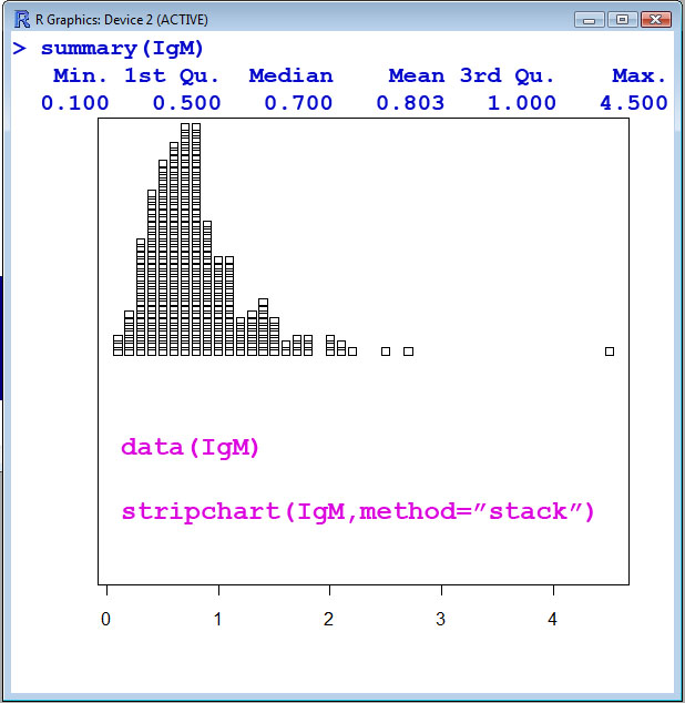
- The IgM data set is only a single column of data, i.e. a single numeric vector or a single variable. The Serum IgM (Immunoglobulin G) level in 298 children ranging in age from 6 months to 6 years. IgM is measured in gram/liter, i.e. g/l for the units.
> library(ISwR)
>
> data(IgM)
>
> stripchart(IgM,method="stack")

> summary(IgM)
   Min. 1st Qu.  Median    Mean 3rd Qu.    Max.
  0.100   0.500   0.700   0.803   1.000   4.500

> sd(IgM)
[1] 0.4694982
>
> mean(IgM)
[1] 0.8030201