Insert Chart toolbar button.

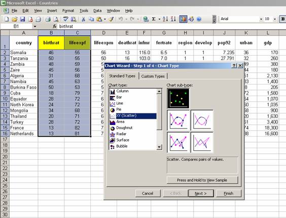
Highlight the columns you wish to create the Chart for first, to make it easier to specify the data you wish to see graphed.

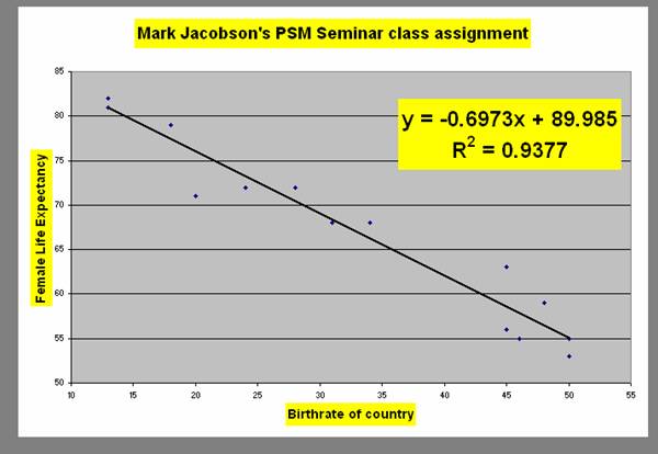
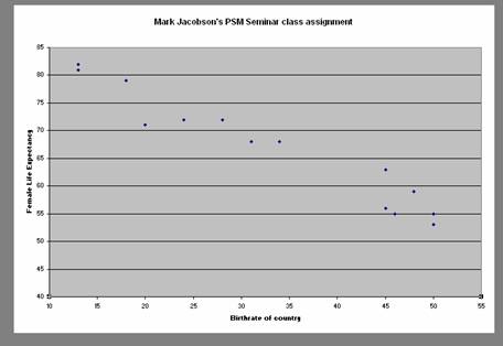
XY (Scatter) is the type of Chart we want. The default sub-type is what is needed for just comparing pairs of values. In this case we will be comparing birthrate and life expectancy of females for each of the 15 countries.

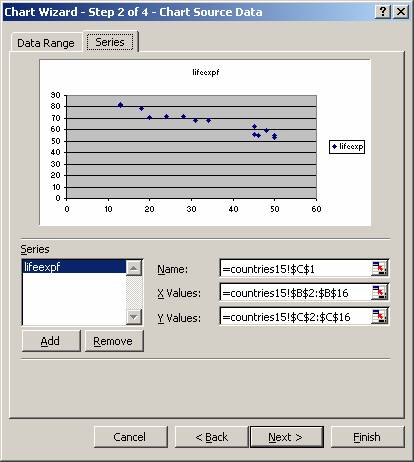
If the X Values Range shown is NOT your independent variable column and/or the Y values Range is NOT your dependent (response) variable column, simply delete the incorrect X values or Y values specification, and then highlight on the worksheet the correct range of values.

For convenience, I have placed the X and the Y variables in consecutive columns on the worksheet, with the dependent X variable to the left of and before the independent Y variable. That will make SPSS guess correctly.

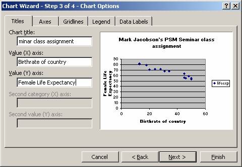
Please put your name on the TITLE, not my name! The legend is NOT NEEDED. Switch to the Legend folder after doing the Chart title, X axis title and Y axis title. Uncheck the check box for Show Legend.

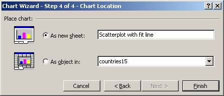
It will be easier just to make a brand new Chart Sheet, instead of placing the chart somewhere in one of your worksheets.

Now you will edit the chart. Double click on the Y axis to get the following dialogue box.

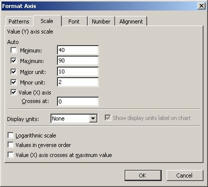
I changed the Minimum to 40 instead of the default 0, for the Scale for the (Y) axis.

By the same method of double clicking on the X-axis, I then changed the Minimum for the X-axis to be 10 instead of 0. You will get something like the following:

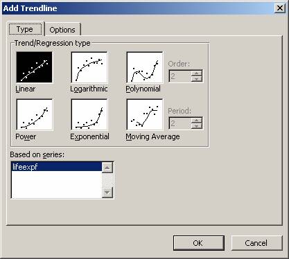
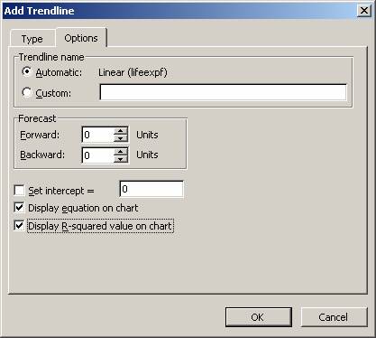
Now it is time to add the Best Fit Line Regression line. Chart menu, Add Trendline is the command that will be available when you have a Chart selected, or when a Chart worksheet is the active worksheet.