See also: Introduction to Information Retrieval, by Christopher D. Manning, Prabhakar Raghavan and Hinrich Schütze

Introduction Example Programs Manipulating the MeSH Vocabulary Program to build a global array index from the NLM MESH (Medical Subject Heading) Hierarchy Program to print all the headings in MESH code order Program that will, when given a keyword, locate the MESH heading containing the keyword and display the full heading, hierarchy codes, and adjacent keywords at this level Make the previous program run as a web server program Indexing the Medical Abstracts Collection OSU Medline Data Base Program to read Medline format abstracts and write out the list of MESH headings for each abstract along with the byte offset of the beginning of the abstract Sort the above and print, for each MESH heading, a count of the number of abstracts it occurs in Miscellaneous Examples Program to compute an optimal binary tree. Dump/restore and data base compression Sorting from Mumps Experimental Data Bases Overview of Searching Boolean Vocabularies Zipf's Law Selection of Indexing Terms Precision and Recall Basic Dictionary Construction WordNet Stop Lists Building a Stop List Vector Space Model Concept Similarity Coeffiecients Example Calculations Related Similarity Functions Experiments Assigning Word Weights Inverse Document Frequency and Basic Vector Space OSU Medline Data Base IDF Weights Wikipedia Data Base IDF Weights Calculating IDF Weights Discrimination Coefficients and Simple Automatic Indexing Basic Retrieval Scanning the doc-term matrix Scanning the term-doc matrix Weighted scanning of the term-doc matrix Scripted test runs Simple Retrieval Faster Simple Retrieval Thesaurus and Phrase Construction Basic Term-Term Co-Occurrence Matrix Modified Basic Indexing - Position Specific Proximity Weighted Term-Term Correlation Matrix Term-Term clutsering Construction of Term Phrases Document-Document Matrices File and Document Clustering Web Page Access N-Gram Experiment Example Code Google Page Rank Algorithm Overview of Other Methods Boolean and Logic Programming Models Conjunctive Normal Form Disjunctive Normal Form Horn Clause Resolution Logic Programming Prolog Vector Space Model Probabilistic Model Fuzzy Set Model Latent Semantic Model Neural Network Model Text Tokens Single Term Based Indexing Phrase Based Indexing N-Gram Based Indexing Methodologies Stemming Algorithms Porter Stemming Algorithm The Lancaster Stemming Algorithm The Lovins stemming algorithm The Krovetz Stemmer Snowball: A language for stemming algorithms Text Searching Boyer Moore String Searching Knuth-Pratt-Morris Algorithm Parsing Visualization Open Directory Indexing and Retrieval of Genetic Text Collections Indexing Text Features in Genomic Repositories Sequence Matching Data Bases Genbank EMBL/EBI Alignment Algorithms Dot Plots Needleman-Wunsch Smith-Waterman Mumps Smith-Waterman Example FASTA BLAST Case Study: Indexing the "nt" Data Base Linguistics and Natural Language Processing Indo-European Languages Miscellaneous Linguistic Links Jakob Grimm Grimm's Law The Clair Library Basic Access Methods 64 Bit Addressing Sequential Random Access Basic Direct Access I/O Indexed Sequential Virtual Sequantial Access Method Key to Address Translation Hash tables Inverted Indices Lists Ordered lists Binary trees Huffman Trees Optimum Weight Balanced Trees Hu-Tucker Trees AVL Trees Tries and Suffix Trees B Trees Data Base Models Networked Data Bases CODASYL Hierarchical Data Bases IMS MUMPS Relational Data Bases Relational Calculus Relational Algebra SQL PostgreSQL MySQL Other Berkeley Data Base (Oracle) Other Topics Soundex Coding Readability Tests MD5 - Message Digest Algorithm 5 Example Javascript Scripts Runnning information retrieval applications through Apache on Windows Data Bases Medical Subject Headings 2003 - mtrees2003.gz OSU-Medline Text - osu-medline.gz WikiPedia Text - wikipedia.txt.gz Experiments Wikipedia Results nohup-wiki-interp-linux nohup-wiki-interp-dos nohup-wiki-combined-dos nohup-wiki-combined-linux wiki.translated.txt.gz wiki.dictionary.sorted.gz wiki.zipf.gz wiki.good.gz wiki.idf.sorted.gz wiki.weighted-doc-vectors.gz wiki.weighted-term-vectors.gz wiki.cohesion.sorted.gz wiki.tt.sorted.gz wiki.jaccard-tt.sorted.gz wiki.dd2.gz wiki.clusters.gz wiki.discrim.sorted.gz wiki.ttfolder.gz sidhe.cs.uni.edu/cgi-bin/wiki/wikiWebFinder.cgi?query=anarchism Web Finder Demo (depends on server availability) sidhe.cs.uni.edu/cgi-bin/wiki/index.cgi?array=lib Folders Demo (depends on server availability). OSU Medline Results (Revised: March 16, 2007) nohup-medline-combined-linux nohup-medline-interp-linux nohup-medline-combined-dos nohup-medline-interp-dos medline.translated.txt.gz medline.dictionary.sorted.gz medline.zipf.gz medline.good.gz medline.idf.sorted.gz medline.weighted-doc-vectors.gz medline.weighted-term-vectors.gz medline.cohesion.sorted.gz medline.tt.sorted.gz medline.jaccard-tt.sorted.gz medline.dd2.gz medline.clusters.gz medline.discrim.sorted.gz medline.ttfolder.gz Web Finder Demo (depends on server availability). Folders Demo (depends on server availability). Computing Text Data Base References

Introduction

The purpose of this text is to illustrate several basic information storage and retrieval techniques through real world data experiments. Information retrieval is the art of identifying similarities between queries and objects in a database. In nearly all cases, the objects found as a result of the query will not be identical to the query but will resemble it in some fashion.

For example, if your query is "give me articles about aviation," the results might include articles about early pioneers in the field, technical reports on aircraft design, flight schedules on airlines, information on airports and so on. For example, the term "aviation" when typed into Google results in about 111,000,000 hits all of which have something to do with aviation.

Information retrieval isn't restricted to text retrieval. So, if you have a cut of a musical piece such as this (from the Beethoven 9th Symphony) and you want to find other music similar to it such as this (from the Beethoven Choral Fantasy), you need a retrieval engine that can detect the similarities, but not von Weber's der Freischutz.

Similar examples exist in many other areas. In Bioinformatics, researchers often identify DNA or protein sequences and search massive databases for similar (and sometimes only distantly related) sequences. For example, the DNA sequence:

>gi|2695846|emb|Y13255.1|ABY13255 Acipenser baeri mRNA for immunoglobulin heavy chain, clone ScH 3.3 TGGTTACAACACTTTCTTCTTTCAATAACCACAATACTGCAGTACAATGGGGATTTTAACAGCTCTCTGTATAATAATGA CAGCTCTATCAAGTGTCCGGTCTGATGTAGTGTTGACTGAGTCCGGACCAGCAGTTATAAAGCCTGGAGAGTCCCATAAA CTGTCCTGTAAAGCCTCTGGATTCACATTCAGCAGCGCCTACATGAGCTGGGTTCGACAAGCTCCTGGAAAGGGTCTGGA ATGGGTGGCTTATATTTACTCAGGTGGTAGTAGTACATACTATGCCCAGTCTGTCCAGGGAAGATTCGCCATCTCCAGAG ACGATTCCAACAGCATGCTGTATTTACAAATGAACAGCCTGAAGACTGAAGACACTGCCGTGTATTACTGTGCTCGGGGC GGGCTGGGGTGGTCCCTTGACTACTGGGGGAAAGGCACAATGATCACCGTAACTTCTGCTACGCCATCACCACCGACAGT GTTTCCGCTTATGGAGTCATGTTGTTTGAGCGATATCTCGGGTCCTGTTGCTACGGGCTGCTTAGCAACCGGATTCTGCC TACCCCCGCGACCTTCTCGTGGACTGATCAATCTGGAAAAGCTTTT

Where the first line identifies the name and library accession numbers of the sequence and the subsequent lines are the DNA nucleotide codes (the letters A, C, G, and T represent Adenine, Cytosine, Guanine, and Thymine, respectively). A program known as BLAST (Basic Local Alignment Sequencing Tool) can be used to find similar sequences in the online databases of known sequences. If you submit the above to NCBI BLAST (National Center for Biotechnology Information), they will conduct a search of their nr database of 6,284,619 nucleotide sequences, presently more than 22,427,755,047 bytes in length. The result is a ranked list of hits of sequences in the data base based on their similarity to the query sequence. Sequences found whose similarity score exceeds a threshold are displayed. One of these is:

>gb|U17058.1|LOU17058 Lepisosteus osseus Ig heavy chain V region mRNA, partial cds Length=159 Score = 151 bits (76), Expect = 4e-33 Identities = 133/152 (87%), Gaps = 0/152 (0%) Strand=Plus/Plus Query 242 TGGGTGGCTTATATTTACTCAGGTGGTAGTAGTACATACTATGCCCAGTCTGTCCAGGGA 301 |||||||| ||||||||| | | ||| || | |||||||||| ||||||||||||||||| Sbjct 4 TGGGTGGCGTATATTTACACCGATGGGAGCAATACATACTATTCCCAGTCTGTCCAGGGA 63 Query 302 AGATTCGCCATCTCCAGAGACGATTCCAACAGCATGCTGTATTTACAAATGAACAGCCTG 361 |||||| |||||||||||||| ||||||| | |||||| ||||| |||| ||||||| Sbjct 64 AGATTCACCATCTCCAGAGACAATTCCAAGAATCAGCTGTACTTACAGATGAGCAGCCTG 123 Query 362 AAGACTGAAGACACTGCCGTGTATTACTGTGC 393 ||||||||||||||||| |||||||||||||| Sbjct 124 AAGACTGAAGACACTGCTGTGTATTACTGTGC 155

In the display from BLAST seen above, the sections of the query that match the sequence in the database are shown. The numbers at the beginning and ends of the lines are the starting and ending points of the subsequence (relative to one, the start of all sequences). Where there are vertical lines between the query and the subject, there is an exact match. Where there are blanks, there was a mismatch.

It should be clear that, even though the subject is different than the query in many places, the two have a high degree of similarity.

Also, consider the search for similar images. Again, this involves searching for similarities, not identity. For example, a human observer would clearly see the two following pictures as dealing with the same subject, despite the differences:

An obvious question would be, how can you write a computer program to see the similarity?

1. Write a program to build a global array indexing vocabulary from the 2003 U.S. NLM MeSH (Medical Subject Heading) Tree Hierarchy. The MeSH codes are used to code medical records and are an ongoing research project of the U.S. National Library of Medicine. The codes used here are from 2003. Newer versions, essentially similar to these, are available from NLM. A local copy of the 2003 MeSH headings is in: 2003 U.S. NLM MeSH (Medical Subject Heading) Tree Hierarchy. Note: this copy is out of date and is used here purely as an example.

   The following is a sample of the MESH tree hierarchy:

   Body Regions;A01 Abdomen;A01.047 Abdominal Cavity;A01.047.025 Peritoneum;A01.047.025.600 Douglas' Pouch;A01.047.025.600.225 Mesentery;A01.047.025.600.451 Mesocolon;A01.047.025.600.451.535 Omentum;A01.047.025.600.573 Peritoneal Cavity;A01.047.025.600.678 Retroperitoneal Space;A01.047.025.750 Abdominal Wall;A01.047.050 Groin;A01.047.365 Inguinal Canal;A01.047.412 Umbilicus;A01.047.849 Back;A01.176 Lumbosacral Region;A01.176.519 Sacrococcygeal Region;A01.176.780 Breast;A01.236 Nipples;A01.236.500 Extremities;A01.378 Amputation Stumps;A01.378.100

   The format is: text description, semi-colon, code hierarchy. Thus, "Body Regions" is code A01, the "Abdomen" is A01.047, the Peritoneum is A01.047.025.600 and so forth. The goal is to build a global array tree where each successive index is a successive code in the MESH hierarchy and the text of each entry is stored in the tree at the appropriate level. Thus, we want something like:

   set ^mesh("A01")="Body Regions" set ^mesh("A01","047")="Abdomen" set ^mesh("A01","047","025")="Abdomenal Cavity" set ^mesh("A01","047","025","600")="Peritoneum" . . . set ^mesh("A01","047","365")="Groin" . . .

   Graphically:

   

   This can be done with a program such as:

   #!/usr/bin/mumps # mtree.mps January 13, 2008 # Copyright 2007 K. C. O'Kane - GPL License applies open 1:"mtrees2003.txt,old" for do . use 1 . read a . if '$test break . set key=$piece(a,";",1) // text description . set code=$piece(a,";",2) // everything else . if key=""!(code="") break . for i=1:1 do .. set x(i)=$piece(code,".",i) // extract code numbers .. if x(i)="" break . set i=i-1 . use 5 . set z="^mesh(" // begin building a global reference #----------------------------------------------------------------------- # build a reference like ^mesh("A01","047","025","600) # by concatenating quotes, codes, quotes, and commas onto z #----------------------------------------------------------------------- . for j=1:1:i-1 set z=z_""""_x(j)_"""," . set z="set "_z_""""_x(i)_""")="""_key_"""" #----------------------------------------------------------------------- # z now looks like set ^mesh("A01","047")="Abdomen" # now execute the text #----------------------------------------------------------------------- . write z,! . xecute z close 1 use 5 write "done",! halt

   Notes:

   • In the program above, for each line of the mesh2003.txt read, a string containing the text of a "set" command like those shown above is created.

   • Note that to embed a double-quote character (") into a string, you place two immediately adjacent double-quote characters into the string. Thus: """" means a string of length one containing a double-quote character.

   • The final string is passed as an argument the xecute` command. The command xecute treats its argument as a line of Mumps code (with limitations, however), and executes it as though it were part of the original program. Execution of this type uses the interpreter and, consequently is much slower than compiled code.

   • Notice the line:

     . if key=""!(code="") break

     uses the OR operator (!). Also note the use of parentheses needed since execution of expressions in Mumps does not rely on precedence.

   • Notice the line:

     . for j=1:1:i-1 set z=z_""""_x(j)_""","

     uses the concatenation operator (_) as well as a local array x(j). Local arrays should be used as little as possible since access to them through the Mumps run-time symbol table can be slow if there are a lot of elements in the symbol table.

   • Notice near the end the close command that releases the file associated with unit 1 and, consequently, makes it available for reuse. Closing a file opened for input is not strictly needed unless you want to reuse the unit number. Closing a file open for output is necessary in order to flush the internal system buffers to disk. If the program crashes before an output file is closed, it is possible to lose data.

   • The output looks like this:

     set ^mesh("A01")="Body Regions" set ^mesh("A01","047")="Abdomen" set ^mesh("A01","047","025")="Abdominal Cavity" set ^mesh("A01","047","025","600")="Peritoneum" set ^mesh("A01","047","025","600","225")="Douglas' Pouch" set ^mesh("A01","047","025","600","451")="Mesentery" set ^mesh("A01","047","025","600","451","535")="Mesocolon" set ^mesh("A01","047","025","600","573")="Omentum" set ^mesh("A01","047","025","600","678")="Peritoneal Cavity" set ^mesh("A01","047","025","750")="Retroperitoneal Space" set ^mesh("A01","047","050")="Abdominal Wall" set ^mesh("A01","047","365")="Groin" set ^mesh("A01","047","412")="Inguinal Canal" set ^mesh("A01","047","849")="Umbilicus" set ^mesh("A01","176")="Back" set ^mesh("A01","176","519")="Lumbosacral Region" set ^mesh("A01","176","780")="Sacrococcygeal Region" set ^mesh("A01","236")="Breast" set ^mesh("A01","236","500")="Nipples" set ^mesh("A01","378")="Extremities" set ^mesh("A01","378","100")="Amputation Stumps" set ^mesh("A01","378","610")="Lower Extremity" set ^mesh("A01","378","610","100")="Buttocks" set ^mesh("A01","378","610","250")="Foot" set ^mesh("A01","378","610","250","149")="Ankle" set ^mesh("A01","378","610","250","300")="Forefoot, Human" set ^mesh("A01","378","610","250","300","480")="Metatarsus" . . .

   • You may print the global ^mesh() data base as follows:

     #!/usr/bin/mumps # mtreeprint.mps January 13, 2008 for lev1=$order(^mesh(lev1)) do . write lev1," ",^mesh(lev1),! . for lev2=$order(^mesh(lev1,lev2)) do .. write ?5,lev2," ",^mesh(lev1,lev2),! .. for lev3=$order(^mesh(lev1,lev2,lev3)) do ... write ?10,lev3," ",^mesh(lev1,lev2,lev3),! ... for lev4=$order(^mesh(lev1,lev2,lev3,lev4)) do .... write ?15,lev4," ",^mesh(lev1,lev2,lev3,lev4),! yields: A01 Body Regions 047 Abdomen 025 Abdominal Cavity 600 Peritoneum 750 Retroperitoneal Space 050 Abdominal Wall 365 Groin 412 Inguinal Canal 849 Umbilicus 176 Back 519 Lumbosacral Region 780 Sacrococcygeal Region 236 Breast 500 Nipples 378 Extremities 100 Amputation Stumps 610 Lower Extremity 100 Buttocks 250 Foot 400 Hip 450 Knee 500 Leg 750 Thigh 800 Upper Extremity 075 Arm 090 Axilla 420 Elbow 585 Forearm 667 Hand 750 Shoulder 456 Head 313 Ear 505 Face 173 Cheek 259 Chin 420 Eye 580 Forehead 631 Mouth 733 Nose 750 Parotid Region 810 Scalp 830 Skull Base 150 Cranial Fossa, Anterior 165 Cranial Fossa, Middle 200 Cranial Fossa, Posterior 598 Neck 673 Pelvis 600 Pelvic Floor 719 Perineum 911 Thorax 800 Thoracic Cavity 500 Mediastinum 650 Pleural Cavity 850 Thoracic Wall 960 Viscera A02 Musculoskeletal System 165 Cartilage 165 Cartilage, Articular 207 Ear Cartilages 410 Intervertebral Disk 507 Laryngeal Cartilages 083 Arytenoid Cartilage 211 Cricoid Cartilage 411 Epiglottis 870 Thyroid Cartilage 590 Menisci, Tibial 639 Nasal Septum 340 Fascia 424 Fascia Lata 513 Ligaments 170 Broad Ligament 514 Ligaments, Articular 100 Anterior Cruciate Ligament 162 Collateral Ligaments 287 Ligamentum Flavum 350 Longitudinal Ligaments 475 Patellar Ligament 600 Posterior Cruciate Ligament . . .

     Alternatively, using some of the newer Mumps functions, the table can be printed as:

     #!/usr/bin/mumps # mtreeprintnew.mps January 28, 2010 set x="^mesh(0)" for do . set x=$query(x) . if x="" break . set i=$qlength(x) . write ?i*2," ",$qsubscript(x,i)," ",@x,?50,x,!

     which produces the output:

     A01 Body Regions ^mesh("A01") 047 Abdomen ^mesh("A01","047") 025 Abdominal Cavity ^mesh("A01","047","025") 600 Peritoneum ^mesh("A01","047","025","600") 225 Douglas' Pouch ^mesh("A01","047","025","600","225") 451 Mesentery ^mesh("A01","047","025","600","451") 535 Mesocolon ^mesh("A01","047","025","600","451","535") 573 Omentum ^mesh("A01","047","025","600","573") 678 Peritoneal Cavity ^mesh("A01","047","025","600","678") 750 Retroperitoneal Space ^mesh("A01","047","025","750") 050 Abdominal Wall ^mesh("A01","047","050") 365 Groin ^mesh("A01","047","365") 412 Inguinal Canal ^mesh("A01","047","412") 849 Umbilicus ^mesh("A01","047","849") 176 Back ^mesh("A01","176") 519 Lumbosacral Region ^mesh("A01","176","519") 780 Sacrococcygeal Region ^mesh("A01","176","780") 236 Breast ^mesh("A01","236") 500 Nipples ^mesh("A01","236","500") 378 Extremities ^mesh("A01","378") 100 Amputation Stumps ^mesh("A01","378","100") 610 Lower Extremity ^mesh("A01","378","610") 100 Buttocks ^mesh("A01","378","610","100") 250 Foot ^mesh("A01","378","610","250") 149 Ankle ^mesh("A01","378","610","250","149") 300 Forefoot, Human ^mesh("A01","378","610","250","300") 480 Metatarsus ^mesh("A01","378","610","250","300","480") 792 Toes ^mesh("A01","378","610","250","300","792") 380 Hallux ^mesh("A01","378","610","250","300","792","380") 510 Heel ^mesh("A01","378","610","250","510") 400 Hip ^mesh("A01","378","610","400") 450 Knee ^mesh("A01","378","610","450") 500 Leg ^mesh("A01","378","610","500") 750 Thigh ^mesh("A01","378","610","750") 800 Upper Extremity ^mesh("A01","378","800") 075 Arm ^mesh("A01","378","800","075") 090 Axilla ^mesh("A01","378","800","090") 420 Elbow ^mesh("A01","378","800","420") 585 Forearm ^mesh("A01","378","800","585") 667 Hand ^mesh("A01","378","800","667") 430 Fingers ^mesh("A01","378","800","667","430") 705 Thumb ^mesh("A01","378","800","667","430","705") 715 Wrist ^mesh("A01","378","800","667","715") 750 Shoulder ^mesh("A01","378","800","750") 456 Head ^mesh("A01","456") 313 Ear ^mesh("A01","456","313") 505 Face ^mesh("A01","456","505") 173 Cheek ^mesh("A01","456","505","173") 259 Chin ^mesh("A01","456","505","259") 420 Eye ^mesh("A01","456","505","420") 338 Eyebrows ^mesh("A01","456","505","420","338") 504 Eyelids ^mesh("A01","456","505","420","504") 421 Eyelashes ^mesh("A01","456","505","420","504","421") 580 Forehead ^mesh("A01","456","505","580") 631 Mouth ^mesh("A01","456","505","631") 515 Lip ^mesh("A01","456","505","631","515")

2. Write a program to print all the headings in MESH code order. Assume the "^mesh()" global array created in the example above. In that example, the keys were organized like this:

   ^mesh("A01") ^mesh("A01","047") ^mesh("A01","047","025") ^mesh("A01","047","025","600") ^mesh("A01","047","025","600","225") ^mesh("A01","047","025","600","451") ^mesh("A01","047","025","600","451","535") ^mesh("A01","047","025","600","573") ^mesh("A01","047","025","600","678") ^mesh("A01","047","025","750") ^mesh("A01","047","050") ^mesh("A01","047","365") ^mesh("A01","047","412") ^mesh("A01","047","849") ^mesh("A01","176")

   with the text of the MeSH code stored at each node.

   This is also the order in which they are stored in the file system. The Mumps function $query() can be used to dump the file system in sequential key order. You pass to $query() a string containing a global array reference (with embedded quotes around string indices). It returns the next array reference in the file system. Eventually, you will run out of "^mesh" references and receive an empty string Consequently, you must test to determine if you received the empty string.

   #!/usr/bin/mumps # meshheadings.mps January 28, 2010 set x="^mesh" // build the first index for do . set x=$query(x) // get next array reference . if x="" break . write x,?50,@x,!

   The output of both of which looks like:

   ^mesh("A01") Body Regions ^mesh("A01","047") Abdomen ^mesh("A01","047","025") Abdominal Cavity ^mesh("A01","047","025","600") Peritoneum ^mesh("A01","047","025","600","225") Douglas' Pouch ^mesh("A01","047","025","600","451") Mesentery ^mesh("A01","047","025","600","451","535") Mesocolon ^mesh("A01","047","025","600","573") Omentum ^mesh("A01","047","025","600","678") Peritoneal Cavity ^mesh("A01","047","025","750") Retroperitoneal Space ^mesh("A01","047","050") Abdominal Wall ^mesh("A01","047","365") Groin ^mesh("A01","047","412") Inguinal Canal ^mesh("A01","047","849") Umbilicus ^mesh("A01","176") Back ^mesh("A01","176","519") Lumbosacral Region ^mesh("A01","176","780") Sacrococcygeal Region ^mesh("A01","236") Breast ^mesh("A01","236","500") Nipples ^mesh("A01","378") Extremities ^mesh("A01","378","100") Amputation Stumps ^mesh("A01","378","610") Lower Extremity ^mesh("A01","378","610","100") Buttocks ^mesh("A01","378","610","250") Foot ^mesh("A01","378","610","250","149") Ankle ^mesh("A01","378","610","250","300") Forefoot, Human ^mesh("A01","378","610","250","300","480") Metatarsus ^mesh("A01","378","610","250","300","792") Toes ^mesh("A01","378","610","250","300","792","380") Hallux ^mesh("A01","378","610","250","510") Heel ^mesh("A01","378","610","400") Hip ^mesh("A01","378","610","450") Knee ^mesh("A01","378","610","500") Leg ^mesh("A01","378","610","750") Thigh ^mesh("A01","378","800") Upper Extremity ^mesh("A01","378","800","075") Arm ^mesh("A01","378","800","090") Axilla ^mesh("A01","378","800","420") Elbow ^mesh("A01","378","800","585") Forearm ^mesh("A01","378","800","667") Hand ^mesh("A01","378","800","667","430") Fingers ^mesh("A01","378","800","667","430","705") Thumb ^mesh("A01","378","800","667","715") Wrist ^mesh("A01","378","800","750") Shoulder

   Notes:

   • the function $query() returns a string containing the next global array reference with indices enclosed in quotes.

   • The line:

           . write x,?50,@x,!
     

     displays the reference (x) and then prints the contents of the node x (@x).

3. Write a program that will, when given a keyword, locate all the MESH headings containing the keyword and display the full heading, hierarchy codes, and adjacent keywords at this level. In effect, this program gives you all the more specific terms related to a higher level, more general term. It locates all instances of the term typed.

   #!/usr/bin/mumps # findmesh.mps January 28, 2010 read "enter keyword: ",key write ! set x="^mesh" // build a global array ref set x=$query(x) if x="" halt for do . if '$find(@x,key) set x=$query(x) // is key stored at this ref? . else do .. set i=$qlength(x) // number of subscripts .. write x," ",@x,! .. for do ... set x=$query(x) ... if x="" halt ... if $qlength(x)'>i break ... write ?5,x," ",@x,! . if x="" halt which yields when given Skeleton as the input: enter keyword: Skeleton ^mesh("A02","835") Skeleton ^mesh("A02","835","232") Bone and Bones ^mesh("A02","835","232","087") Bones of Upper Extremity ^mesh("A02","835","232","087","144") Carpal Bones ^mesh("A02","835","232","087","144","650") Scaphoid Bone ^mesh("A02","835","232","087","144","663") Semilunar Bone ^mesh("A02","835","232","087","227") Clavicle ^mesh("A02","835","232","087","412") Humerus ^mesh("A02","835","232","087","535") Metacarpus ^mesh("A02","835","232","087","702") Radius ^mesh("A02","835","232","087","783") Scapula ^mesh("A02","835","232","087","783","261") Acromion ^mesh("A02","835","232","087","911") Ulna ^mesh("A02","835","232","169") Diaphyses ^mesh("A02","835","232","251") Epiphyses ^mesh("A02","835","232","251","352") Growth Plate ^mesh("A02","835","232","300") Foot Bones ^mesh("A02","835","232","300","492") Metatarsal Bones ^mesh("A02","835","232","300","710") Tarsal Bones ^mesh("A02","835","232","300","710","300") Calcaneus ^mesh("A02","835","232","300","710","780") Talus ^mesh("A02","835","232","409") Hyoid Bone ^mesh("A02","835","232","500") Leg Bones ^mesh("A02","835","232","500","247") Femur ^mesh("A02","835","232","500","247","343") Femur Head ^mesh("A02","835","232","500","247","510") Femur Neck ^mesh("A02","835","232","500","321") Fibula ^mesh("A02","835","232","500","624") Patella ^mesh("A02","835","232","500","883") Tibia ^mesh("A02","835","232","611") Pelvic Bones ^mesh("A02","835","232","611","108") Acetabulum ^mesh("A02","835","232","611","434") Ilium ^mesh("A02","835","232","611","548") Ischium ^mesh("A02","835","232","611","781") Pubic Bone ^mesh("A02","835","232","730") Sesamoid Bones ^mesh("A02","835","232","781") Skull ^mesh("A02","835","232","781","200") Cranial Sutures ^mesh("A02","835","232","781","292") Ethmoid Bone ^mesh("A02","835","232","781","324") Facial Bones ^mesh("A02","835","232","781","324","502") Jaw ^mesh("A02","835","232","781","324","502","125") Alveolar Process ^mesh("A02","835","232","781","324","502","125","800") Tooth Socket ^mesh("A02","835","232","781","324","502","320") Dental Arch ^mesh("A02","835","232","781","324","502","632") Mandible ^mesh("A02","835","232","781","324","502","632","130") Chin ^mesh("A02","835","232","781","324","502","632","600") Mandibular Condyle ^mesh("A02","835","232","781","324","502","645") Maxilla ^mesh("A02","835","232","781","324","502","660") Palate, Hard ^mesh("A02","835","232","781","324","665") Nasal Bone ^mesh("A02","835","232","781","324","690") Orbit ^mesh("A02","835","232","781","324","948") Turbinates ^mesh("A02","835","232","781","324","995") Zygoma ^mesh("A02","835","232","781","375") Frontal Bone ^mesh("A02","835","232","781","572") Occipital Bone ^mesh("A02","835","232","781","572","434") Foramen Magnum ^mesh("A02","835","232","781","651") Parietal Bone ^mesh("A02","835","232","781","750") Skull Base ^mesh("A02","835","232","781","750","150") Cranial Fossa, Anterior ^mesh("A02","835","232","781","750","165") Cranial Fossa, Middle ^mesh("A02","835","232","781","750","400") Cranial Fossa, Posterior ^mesh("A02","835","232","781","802") Sphenoid Bone ^mesh("A02","835","232","781","802","662") Sella Turcica ^mesh("A02","835","232","781","885") Temporal Bone ^mesh("A02","835","232","781","885","444") Mastoid ^mesh("A02","835","232","781","885","681") Petrous Bone ^mesh("A02","835","232","834") Spine ^mesh("A02","835","232","834","151") Cervical Vertebrae ^mesh("A02","835","232","834","151","213") Atlas ^mesh("A02","835","232","834","151","383") Axis ^mesh("A02","835","232","834","151","383","668") Odontoid Process ^mesh("A02","835","232","834","229") Coccyx ^mesh("A02","835","232","834","432") Intervertebral Disk ^mesh("A02","835","232","834","519") Lumbar Vertebrae ^mesh("A02","835","232","834","717") Sacrum ^mesh("A02","835","232","834","803") Spinal Canal ^mesh("A02","835","232","834","803","350") Epidural Space ^mesh("A02","835","232","834","892") Thoracic Vertebrae ^mesh("A02","835","232","904") Thorax ^mesh("A02","835","232","904","567") Ribs ^mesh("A02","835","232","904","766") Sternum ^mesh("A02","835","232","904","766","442") Manubrium ^mesh("A02","835","232","904","766","825") Xiphoid Bone ^mesh("A02","835","583") Joints ^mesh("A02","835","583","032") Acromioclavicular Joint ^mesh("A02","835","583","097") Atlanto-Axial Joint ^mesh("A02","835","583","101") Atlanto-Occipital Joint ^mesh("A02","835","583","156") Bursa, Synovial ^mesh("A02","835","583","192") Cartilage, Articular ^mesh("A02","835","583","290") Elbow Joint ^mesh("A02","835","583","345") Finger Joint ^mesh("A02","835","583","345","512") Metacarpophalangeal Joint ^mesh("A02","835","583","378") Foot Joints ^mesh("A02","835","583","378","062") Ankle Joint ^mesh("A02","835","583","378","531") Metatarsophalangeal Joint ^mesh("A02","835","583","378","831") Tarsal Joints ^mesh("A02","835","583","378","831","780") Subtalar Joint ^mesh("A02","835","583","378","900") Toe Joint ^mesh("A02","835","583","411") Hip Joint ^mesh("A02","835","583","443") Joint Capsule ^mesh("A02","835","583","443","800") Synovial Membrane ^mesh("A02","835","583","443","800","800") Synovial Fluid ^mesh("A02","835","583","475") Knee Joint ^mesh("A02","835","583","475","590") Menisci, Tibial ^mesh("A02","835","583","512") Ligaments, Articular ^mesh("A02","835","583","512","100") Anterior Cruciate Ligament ^mesh("A02","835","583","512","162") Collateral Ligaments ^mesh("A02","835","583","512","162","500") Lateral Ligament, Ankle ^mesh("A02","835","583","512","162","600") Medial Collateral Ligament, Knee ^mesh("A02","835","583","512","287") Ligamentum Flavum ^mesh("A02","835","583","512","350") Longitudinal Ligaments ^mesh("A02","835","583","512","475") Patellar Ligament ^mesh("A02","835","583","512","600") Posterior Cruciate Ligament ^mesh("A02","835","583","656") Pubic Symphysis ^mesh("A02","835","583","707") Sacroiliac Joint ^mesh("A02","835","583","748") Shoulder Joint ^mesh("A02","835","583","781") Sternoclavicular Joint ^mesh("A02","835","583","790") Sternocostal Joints ^mesh("A02","835","583","861") Temporomandibular Joint ^mesh("A02","835","583","861","900") Temporomandibular Joint Disk ^mesh("A02","835","583","959") Wrist Joint ^mesh("A02","835","583","979") Zygapophyseal Joint ^mesh("A11","284","295","154","200") Cell Wall Skeleton ^mesh("D12","776","097","162") Cell Wall Skeleton ^mesh("D12","776","395","560","186") Cell Wall Skeleton ^mesh("E01","370","350","700","050") Age Determination by Skeleton

   Notes:

   • Read in the keyword. Build in a string a global array reference containing the first key: ^mesh and locate the first indices of this array with $query().

   • In a loop, get the text value stored at the global array reference and check to see if it contains the keyword that was typed. This is done by the line below reading:

     . if $find(@x,key) do  // is key stored at this ref?
     

     which uses indirection to get the text value stored (@x evaluates to the contents of the global array reference in x). The $find() function searches the text for any substring containing the input key.

   • If $find() does not find the key, the next global array reference is found with $query(). The value returned by $query() is checked that it is not empty. If not, the loop continues with the next reference to the array "^mesh".

   • If the key word is found in the text, print the reference and scan for additional references whose number of subscripts is greater than that of the found reference (sub tress of the found reference). The function $qlength() returns the number of subscripts in a reference.

4. Make the previous program run as a web server information storage and retrieval application.

   HTML file query3.html: <html> <head> <title> Example server side Mumps Program</title> </head> <body bgcolor=silver> Enter a MeSH term: &nbsp; <form method="get" action=cgi-bin/isr.mps> <input type=text size=30 name=key value="Head"> &nbsp; <input type=submit> </form> </body> </html>

   Next move the following file to ~/public_html/cgi-bin and make it world readable and executable.

   #!/usr/bin/mumps # isr.mps January 28, 2010 html Content-type: text/html &!&! html <html><body bgcolor=silver> if '$data(key) write "No keyword supplied</body></html>",! halt html <center>Results for &~key~</center><hr> html <pre> set x="^mesh" // build a global array ref set x=$query(x) if x="" halt for do . if '$find(@x,key) set x=$query(x) // is key stored at this ref? . else do .. set i=$qlength(x) // number of subscripts .. write x," ",@x,! .. for do ... set x=$query(x) ... if x="" write "</pre></body></html>",! halt ... if $qlength(x)'>i break ... write ?5,x," ",@x,! . if x="" write "</pre></body></html>",! halt

   Now copy mtree.mps and mtrees2003.txt to /var/www/cgi-bin. Run mtree.mps then make the database files key.dat and data.dat world readable and world writable. These now contain the MESH data base that the server side query program isr.mps will access.

   Some notes:

   • The HTML file isr.html sets up an HTML form that can be used to collect information. The FORM tag allows for single line text, a box of text, radio buttons, check boxes and selection lists (drop down boxes). Each item of data collected, upon clicking the SUBMIT button, is placed into a URL and sent to the web server. In this example, only a line of text is collected.

   • The "value" strings are encoded as follows by the browser: alphabetics and numerics remain unchanged; blanks become plus signs and all other characters appear in the form %XX where XX is a hexadecimal number indicating the character's collating sequence value. If more than one name=value figures is appended to the URL, they, are separated from one another by and ampersand (&).

   • The interpreter automatically reads QUERY_STRING (which contains the parameters following the question mark) and decodes them. For each "name" found, it creates a variable of the same name in the Mumps run-time symbol table initialized to the "value" field. Names should be unique although non-unique names can be handled (see the manual).

   • When your CGI program runs, its output is captured by the web server and sent back to the originating browser. The first thing you send to the web server MUST be the line:

     
     html Content-type: text/html &!&!
     
     

     exactly as typed. This tells the web server what's coming next. After this line, everything sent would be in HTML format. The Mumps command "html" is an output command that causes the remainder of the line to be written to the web server. Write commands can also be used but the text requires a lot of annoying quote marks. You may embed in the HTML line figures of the form:

     &!  and &~expression~
     

     The first of these, &!, causes a new line. The second causes evaluation of the expression and the result to be written to the web server (the &~ and ~ are not sent).

   Now open a browser and enter:

   
   127.0.0.1/cgi-bin/isr.html
   
   

   This will bring up the first screen shown below. Click Submit and the second screen will appear.

   

   

5. The following code illustrates most of the major FORM data collection techniques:

   <form method="get" action="quiz2.cgi"> <center> Name: <input type="text" name="name" size=40 value=""><br> </center> Class: <input type="Radio" name="class" value="freshman" > Freshman <input type="Radio" name="class" value="sophomore" > Sophomore <input type="Radio" name="class" value="junior" > Junior <input type="Radio" name="class" value="senior" checked> Senior <input type="Radio" name="class" value="grad" > Grad Student <br> Major: <select name="major" size=7> <option value="computer science" >computer science <option value="mathematics" >Mathematics <option value="biology" selected>Biology <option value="chemistry" >Chemistry <option value="earth science" >Earth Science <option value="industrial technology" >Industrial Technology <option value="physics" >Physics </select> <table border> <tr> <td valign=top> Hobbies: </td> <td> <input type="Checkbox" name="hobby1" value="stamp collecting" > Stamp Collecting<br> <input type="Checkbox" name="hobby2" value="art" > Art<br> <input type="Checkbox" checked name="hobby3" value="bird watching" > Bird Watching<br> <input type="Checkbox" name="hobby4" value="hang gliding" > Hang Gliding<br> <input type="Checkbox" name="hobby5" value="reading" > Reading<br> </td></tr> </table> <center> <input type="submit" value="go for it"> </center> </form>

   which produces:

   

   Click here for a good synopsis of HTML commands.

6. OSU Medline Data Base

   The text (which will be used in subsequent examples) OSU Medline Data Base based on the TREC-9 conference. TREC (Text REtrieval Conferences) are annual events sponsored by the National Institute for Standards and Technology (NIST). Past data sets are at http://trec.nist.gov/data.html The TREC-9 Filtering Track data base consisted of a collection of medically related titles and abstracts:

   "... The OHSUMED test collection is a set of 348,566 references from MEDLINE, the on-line medical information database, consisting of titles and/or abstracts from 270 medical journals over a five-year period (1987-1991). The available fields are title, abstract, MeSH indexing terms, author, source, and publication type. The National Library of Medicine has agreed to make the MEDLINE references in the test database available for experimentation, restricted to the following conditions: 1. The data will not be used in any non-experimental clinical, library, or other setting. 2. Any human users of the data will explicitly be told that the data is incomplete and out-of-date. The OHSUMED document collection was obtained by William Hersh (hersh@OHSU.EDU) and colleagues for the experiments described in the papers below: Hersh WR, Buckley C, Leone TJ, Hickam DH, OHSUMED: An interactive retrieval evaluation and new large test collection for research, Proceedings of the 17th Annual ACM SIGIR Conference, 1994, 192-201. Hersh WR, Hickam DH, Use of a multi-application computer workstation in a clinical setting, Bulletin of the Medical Library Association, 1994, 82: 382-389. ..."

   Data from the OHSUMED file were modified and edited into a format similar to that currently used by MEDLINE in order to present a more easily managed file. The original format used many very long lines which were inconvenient to manipulate as well as a number of fields that were not of interest for this study. The conversion programs are given in the experimental data bases section below. The revised data base has the following appearance:

   STAT- MEDLINE MH Acetaldehyde/*ME MH Buffers MH Catalysis MH HEPES/PD MH Nuclear Magnetic Resonance MH Phosphates/*PD MH Protein Binding MH Ribonuclease, Pancreatic/AI/*ME MH Support, U.S. Gov't, Non-P.H.S. MH Support, U.S. Gov't, P.H.S. TI The binding of acetaldehyde to the active site of ribonuclease: alterations in catalytic ... AB Ribonuclease A was reacted with [1-13C,1,2-14C]acetaldehyde and sodium cyanoborohydride in the presence or absence of 0.2 M phosphate. After several hours of incubation at 4 degrees C (pH 7.4) stable acetaldehyde-RNase adducts were formed, and the extent of their formation was similar regardless of the presence of phosphate. Although the total amount of covalent binding was comparable in the absence or presence of phosphate, this active site ligand prevented the inhibition of enzymatic activity seen in its absence. This protective action of phosphate diminished with progressive ethylation of RNase, indicating that the reversible association of phosphate with the active site lysyl residue was overcome by the irreversible process of reductive ethylation. Modified RNase was analysed using 13C proton decoupled NMR spectroscopy. Peaks arising from the covalent binding of enriched acetaldehyde to free amino groups in the absence of phosphate were as follows: NH2-terminal alpha amino group, 47.3 ppm; bulk ethylation at epsilon amino groups of nonessential lysyl residues, 43.0 ppm; and the epsilon amino group of lysine-41 at the active site, 47.4 ppm. In the spectrum of RNase ethylated in the presence of phosphate, the peak at 47.4 ppm was absent. When RNase was selectively premethylated in the presence of phosphate, to block all but the active site lysyl residues and then ethylated in its absence, the signal at 43.0 ppm was greatly diminished, and that arising from the active site lysyl residue at 47.4 ppm was enhanced. These results indicate that phosphate specifically protected the active site lysine from reaction with acetaldehyde, and that modification of this lysine by acetaldehyde adduct formation resulted in inhibition of catalytic activity. STAT- MEDLINE MH Adult MH Alcohol, Ethyl/*AN MH Breath Tests/* MH Human MH Irrigation MH Male MH Middle Age MH Mouth/* MH Temperature MH Water TI Reductions in breath ethanol readings in normal male volunteers following mouth ... AB Blood ethanol concentrations were measured sequentially, over a period of hours, using a Lion AE-D2 alcolmeter, in 12 healthy male subjects given oral ethanol 0.5 g/kg body wt. Readings were taken before and after rinsing the mouth with water at varying temperatures. Mouth rinsing resulted in a reduction in the alcolmeter readings at all water temperatures tested. The magnitude of the reduction was greater after rinsing with water at lower temperatures. This effect occurs because rinsing cools the mouth and dilutes retained saliva. This finding should be taken into account whenever breath analysis is used to estimate blood ethanol concentrations in experimental situations. . . . (Note: long lines truncated from the above)

7. Write a program to read Medline format abstracts (from the modified TREC-9 data base described above) and write out a list of MESH headings, the number of times each occurs, and the title of each abstract in which it occurs along with the byte offset of the abstract in the master file.

   The lines with text MeSH headings in the data base have the code MH in positions one and 2. There is a blank line that signals the end of each abstract. Offsets are the byte offset relative to the start of the file where the entry for the abstract and related material began. This number can be used to retrieve the entry. Place # between the text and the offset. The figure # does not exists as text in any MeSH heading and can be used as a separator when the file is subsequently read.

   #!/usr/bin/mumps # readmedline.mps January 28, 2010 open 1:"osu.medline,old" use 1 set x=0 // a counter to limit the size set i=$ztell // return the integer offset in the file for do . use 1 . read a . if '$test break # if a blank line, record the offset - this is the start of an abstract . if a="" set i=$ztell set x=x+1 break:x>10000 quit // return the offset in the file . if $extract(a,1,3)="MH " do .. use 5 .. set a=$piece($extract(a,7,255),"/",1) .. write a,"#",i,!

   A portion of the output from which is:

   Acetaldehyde#0 Buffers#0 Catalysis#0 HEPES#0 Nuclear Magnetic Resonance#0 Phosphates#0 Protein Binding#0 Ribonuclease, Pancreatic#0 Support, U.S. Gov't, Non-P.H.S.#0 Support, U.S. Gov't, P.H.S.#0 Adult#2401 Alcohol, Ethyl#2401 Breath Tests#2401 Human#2401 Irrigation#2401 Male#2401 Middle Age#2401 Mouth#2401 Temperature#2401 Water#2401 Alcoholism#3479 Animal#3479 Diprenorphine#3479 Female#3479 Morphine#3479 Naloxone#3479 Naltrexone#3479 Narcotic Antagonists#3479 Rats#3479 Rats, Inbred Strains#3479 Receptors, Endorphin#3479 Seizures#3479 Substance Withdrawal Syndrome#3479 Adult#4510 Alcohol Drinking#4510 Alcoholism#4510 Erythrocyte Indices#4510

   Notes:

   • The function $ztell gives the byte offset of the current file.

   • Some MeSH headings have extraneous text following the main code and separated from the main code by a "/" character. Only text prior to and "/" character is extracted. The $piece() function returns either the entire string or, if "/" is present, just the part of the string prior to "/".

8. Sort the output of the above and print, for each MESH heading, a count of the number of abstracts it occurs in along with the titles of the documents containing it using the command:

   readmedline.mps | sortmedline.mps > words

   #!/usr/bin/mumps # sortmedline.mps January 28, 2010 open 1:"osu.medline,old" if '$test write "file open error",! halt kill ^MH for do . read a . if '$test break . set b=$piece(a,"#") // get MH word(s) . set c=$piece(a,"#",2) // get file offset # create or increment entry for word . if $data(^MH(b)) set ^MH(b)=^MH(b)+1 . else set ^MH(b)=1 # store the offset . set ^MH(b,c)="" // store the offset # write for each heading the titles associated with it set x="" for do . set x=$order(^MH(x)) . if x="" break . write x," occurs in ",^MH(x)," documents",! . for off=$order(^MH(x,off)) do .. use 1 .. do $zseek(off) // move to location in file .. for do // scan input lines for title line ... read a ... if $extract(a,1,3)'="TI " quit ... use 5 ... write ?5,off,?15,$extract(a,7,80),! ... break

   The output of which looks like:

   Abdominal Injuries occurs in 13 documents 1650173 Percutaneous transcatheter steel-coil embolization of a large proximal pos 1678059 Features of 164 bladder ruptures. 2523966 Injuries to the abdominal vascular system: how much does aggressive resusc 3436121 Triple-contrast computed tomography in the evaluation of penetrating poste 4624903 Correlations of injury, toxicology, and cause of death to Galaxy Flight 20 4901771 Selective management of blunt abdominal trauma in children--the triage rol 4913645 Percutaneous peritoneal lavage using the Veress needle: a preliminary repo 6713150 The seat-belt syndrome. 7019763 Early diagnosis of shock due to pericardial tamponade using transcutaneous 7885247 The incidence of severe trauma in small rural hospitals. 8189154 Intussusception following abdominal trauma. 8808690 Hepatic and splenic injury in children: role of CT in the decision for lap 8961708 Peritoneal lavage and the surgical resident. Abdominal Neoplasms occurs in 6 documents 10033669 Current spectrum of intestinal obstruction. 10399042 Diagnosis of metastases from testicular germ cell tumours using fine needl 116380 Intracystic injection of OK-432: a new sclerosing therapy for cystic hygro 5804499 Pheochromocytoma, polycythemia, and venous thrombosis. 8983032 Malignant epithelioid peripheral nerve sheath tumor arising in a benign sc 8991187 DTIC therapy in patients with malignant intra-abdominal neuroendocrine tum Abdominal Wall occurs in 11 documents 10291646 Structure of abdominal muscles in the hamster: effect of elastase-induced 2142543 Surgical incision for cesarean section. 2230059 Exstrophy, epispadias, and cloacal and urogenital sinus abnormalities. 2963791 Adductor tendinitis and musculus rectus abdominis tendopathy. 5426490 Postpartum sit-ups [letter] 5438957 Bilateral upper-quadrant (intercostal) flaps: the value of protective sens 6012451 Anterior rectus sheath repair for inguinal hernia. 6557458 Effects of upper or lower abdominal surgery on diaphragmatic function. 8946400 Patterns of muscular activity during movement in patients with chronic low 8947451 Trunk muscle balance and muscular force. 9892904 Venous plasma (total) bupivacaine concentrations following lower abdominal

   Write a program to compute an optimal binary tree. See this link

   read "n " n for i=1:1:n do . write "p",i," " . read p(i) for i=0:1:n do . write "q",i," " . read q(i) for i=0:1:n do . for j=0:1:n do .. set r(i,j)=0 for i=0:1:n do . set c(i,i)=0 . set w(i,i)=q(i) . for j=i+1:1:n do .. if j'>n set w(i,j)=w(i,j-1)+p(j)+q(j) for j=1:1:n do . set c(j-1,j)=w(j-1,j),r(j-1,j)=j for d=2:1:n do . for j=d:1:n do .. set i=j-d,y=r(i,j-1) .. set x=c(i,y-1)+c(y,j) .. do xx .. set c(i,j)=w(i,j)+x,r(i,j)=y write !,"matrix",! for m=0:1:n-1 do . write ! . for l=1:1:n do .. write r(m,l)," " write !,! set s=1 set s(s)=0_","_n set c=1 set nx=2 set a(1)="b(0" y if $piece(s(c),",",1)-$piece(s(c),",",2)=0 do . set c=c+1 . if c<nx goto y . goto z set s(nx)=$piece(s(c),",",1)_","_(r(@s(c))-1) set a(nx)=a(c)_",1" set nx=nx+1 set s(nx)=r(@s(c))_","_$p(s(c),",",2) set a(nx)=a(c)_",2" set nx=nx+1 set c=c+1 goto y z for i=1:1:c-1 do . set a(i)=a(i)_")" for i=1:1:c-1 do . write a(i),!,s(i),! . set @a(i)=r(@s(i)) for i=1:1:c-1 do . write !,a(i),"->",@a(i) halt xx for k=r(i,j-1):1:r(i+1,j) do . if c(i,k-1)+c(k,j)<x do .. set x=c(i,k-1)+c(k,j) .. set y=k quit which when given input: n 7 p1 2 p2 3 p3 2 p4 4 p5 2 p6 3 p7 2 q0 1 q1 1 q2 1 q3 1 q4 1 q5 1 q6 1 q7 1 writes: matrix 1 2 2 2 4 4 4 0 2 2 3 4 4 4 0 0 3 4 4 4 4 0 0 0 4 4 5 6 0 0 0 0 5 6 6 0 0 0 0 0 6 6 0 0 0 0 0 0 7 b(0) 0,7 b(0,1) 0,3 b(0,2) 4,7 b(0,1,1) 0,1 b(0,1,2) 2,3 b(0,2,1) 4,5 b(0,2,2) 6,7 b(0,1,1,1) 0,0 b(0,1,1,2) 1,1 b(0,1,2,1) 2,2 b(0,1,2,2) 3,3 b(0,2,1,1) 4,4 b(0,2,1,2) 5,5 b(0,2,2,1) 6,6 b(0,2,2,2) 7,7 b(0)->4 b(0,1)->2 b(0,2)->6 b(0,1,1)->1 b(0,1,2)->3 b(0,2,1)->5 b(0,2,2)->7 b(0,1,1,1)->0 b(0,1,1,2)->0 b(0,1,2,1)->0 b(0,1,2,2)->0 b(0,2,1,1)->0 b(0,2,1,2)->0 b(0,2,2,1)->0 b(0,2,2,2)->0

   Dump/restore and data base compression

   As is the case with many data base systems, once disk blocks have been allocated, they remain as permanent parts of the file system, even if, due to deletions, they are no longer needed. In some system, this results in an accumulation of unused blocks. In a B-tree based system such as used in Mumps, block occupancy can vary considerably after many deletions and reorganizations. In order to remove unused blocks and rebuild the B-tree with blocks that are mostly half filled, the data base should be dumped to a sequential, collated ASCII file, the old data base (key.dat and data.dat) erased and then the data base restored from the ACSII file.

   There are two functions in Mumps to accomplish this: $zcd() and $zcl(). The first of these, $zcd() writes the full data base to disk as an ASCII file. If given a string parameter, it will use the contents of the string as the file name. If no file name is given, the default will be the system time in seconds followed by ".dmp". The second function, $zcl() restores the data base. If given a file name parameter, it will load from the file specified. If no parameter is given, it will look for a file named "dump".

   For example, in a large run of 25,000 abstracts which included creation and pruning of the ^doc(), ^index(), ^idf(), ^mca(), ^df() and ^dict() vectors as well as creation of ^tt() and ^dd() matrices, the global array data base was:

   -rw-rw-rw-    1 root     root          19M Mar  5 04:40 /d1/isr/code/data.dat
   -rw-rw-rw-    1 root     root         262M Mar  5 04:40 /d1/isr/code/key.dat
   

   After a dump/restore cycle it was:

   -rw-rw-rw-    1 root     root         8.5M Mar  5 09:52 data.dat
   -rw-rw-rw-    1 root     root         107M Mar  5 09:52 key.dat
   

   The intermediate dump file was 38M bytes in length. In this case, the dump/restore resulted in more than 2 to 1 in savings and, consequently, faster access due to fewer blocks searched. The following are the steps:

   run the program: #!/usr/bin/mumps # # dump the data base # do $zcd followed by the system command: mv 11100370.dmp dump which renames the dump data set, followed by the system commands: rm key.dat rm data.dat which delete the old data sets, followed by running the program: #!/usr/bin/mumps # # restore the data base # do $zcl which reloads and rebuilds the data base.

   Dump/restore routines can be used to create backup copies of a data base for later restoration. A dump/restore is generally very quick, taking only a few minutes (depending on file size). This is due to the relatively sequential nature of the B-tree load.

   Sorting from Mumps

   The easiest way to sort is to write out a file, close it, and then invoke the system "sort" program. For example, suppose you have a vector of words containing their frequency of occurrence (^dict) and you want to order them by frequency of occurrence. The vector itself is ordered alphabetically by word, the primary index. You can produce a list sorted by frequency with the following:

   #!/usr/bin/mumps open 1:"temp.dat,new" use 1 for w=$order(^dict(w)) do . write ^dict(w)," ",w,! use 5 close 1 set i=$zsystem("sort -n < temp.dat > temp1.dat") // -n means numeric if i!=0 do . write "sort failed",! . shell rm temp.dat temp1.dat . halt open 1:"temp1.dat,old" for do . use 1 read line . if !$test break . use 5 write line,! use 5 close 1 shell rm temp.dat temp1.dat

   While it is possible to use global arrays to sort, it is generally a bad idea. The system sort program is much faster and more efficient. The sort program has many options, such as the -n (numeric sort) shown above. These include the ability to sort ascending, descending and on multiple fields. See the documentation by typing "man sort" on a Linux or Unix system.

1. Experimental Data Bases

   For some of the experiments below, the OHSUMED TREC-9 data base was used. The OHSUMED test collection is a set of 348,566 references from Medline, the on-line medical information database, consisting of titles and/or abstracts from 270 medical journals over a five-year period (1987-1991). The data base was filtered and reformatted to conform to the style similar to that used by online NLM Medline abstracts. A compressed, filtered copy of the reformatted data base is here.

   The original text had the following appearance:

   .I 1 .U 87049087 .S Am J Emerg Med 8703; 4(6):491-5 .M Allied Health Personnel/*; Electric Countershock/*; Emergencies; Emergency Medical Technicians/*; Human; Prognosis; R ecurrence; Support, U.S. Gov't, P.H.S.; Time Factors; Transportation of Patients; Ventricular Fibrillation/*TH. .T Refibrillation managed by EMT-Ds: incidence and outcome without paramedic back-up. .P JOURNAL ARTICLE. .W Some patients converted from ventricular fibrillation to organized rhythms by defibrillation-trained ambulance techni cians (EMT-Ds) will refibrillate before hospital arrival. The authors analyzed 271 cases of ventricular fibrillation managed by EMT-Ds working without paramedic back-up. Of 111 patients initially converted to organized rhythms, 19 (17 %) refibrillated, 11 (58%) of whom were reconverted to perfusing rhythms, including nine of 11 (82%) who had spontane ous pulses prior to refibrillation. Among patients initially converted to organized rhythms, hospital admission rates were lower for patients who refibrillated than for patients who did not (53% versus 76%, P = NS), although discharge rates were virtually identical (37% and 35%, respectively). Scene-to-hospital transport times were not predictively associated with either the frequency of refibrillation or patient outcome. Defibrillation-trained EMTs can effectivel y manage refibrillation with additional shocks and are not at a significant disadvantage when paramedic back-up is no t available. .A Stults KR; Brown DD.

   The C++ filtering program is:

   # cvtosu.cpp March 5, 2005 #include #include int main() { char line[8192]; long i,j,k; long acc=0; int first=1; while (1) { if (fgets(line,8192,stdin)==NULL) break; i=strlen(line); line[i-1]='\0'; if (strncmp(line,".I",2)==0) { if (!first) cout << endl; first=0; cout << "STAT- MEDLINE" << endl; continue; } if (strncmp(line,".T",2)==0) { acc++; fgets(line,8192,stdin); i=strlen(line); line[i-1]='\0'; // remove newline j=0; cout << "TI " << line << endl; continue; } if (strncmp(line,".W",2)==0) { fgets(line,8192,stdin); cout << "AB "; i=strlen(line); line[i-1]='\0'; // remove newline j=0; for (i=0; line[i]!=0; i++) { cout << line[i]; j++; if (j>50 && line[i]==' ') { cout << endl << " "; j=0; } } cout << endl; } if (strncmp(line,".M",2)==0) { char word[512]; fgets(line,8192,stdin); i=strlen(line); line[i-2]='\0'; word[0]=0; while (1) { for (j=0; line[j]!=0; j++) { if (line[j]==';') break; word[j]=line[j]; } word[j]=0; cout << "MH " << word << endl; if (line[j]==0) break; j++; if (line[j]==0) break; while (line[j]==' ') j++; strcpy(line,&line[j]); if (line[0]==0) break; } } } return 1; } which produces text of the format: STAT- MEDLINE MH Acetaldehyde/*ME MH Buffers MH Catalysis MH HEPES/PD MH Nuclear Magnetic Resonance MH Phosphates/*PD MH Protein Binding MH Ribonuclease, Pancreatic/AI/*ME MH Support, U.S. Gov't, Non-P.H.S. MH Support, U.S. Gov't, P.H.S. TI The binding of acetaldehyde to the active site of ribonuclease: alterations in catalytic activity and AB Ribonuclease A was reacted with [1-13C,1,2-14C]acetaldehyde and sodium cyanoborohydride in the presence or absence of 0.2 M phosphate. After several hours of incubation at 4 degrees C (pH 7.4) stable acetaldehyde-RNase adducts were formed, and the extent of their formation was similar regardless of the presence of phosphate. Although the total amount of covalent binding was comparable in the absence or presence of phosphate, this active site ligand prevented the inhibition of enzymatic activity seen in its absence. This protective action of phosphate diminished with progressive ethylation of RNase, indicating that the reversible association of phosphate with the active site lysyl residue was overcome by the irreversible process of reductive ethylation. Modified RNase was analysed using 13C proton decoupled NMR spectroscopy. Peaks arising from the covalent binding of enriched acetaldehyde to free amino groups in the absence of phosphate were as follows: NH2-terminal alpha amino group, 47.3 ppm; bulk ethylation at epsilon amino groups of nonessential lysyl residues, 43.0 ppm; and the epsilon amino group of lysine-41 at the active site, 47.4 ppm. In the spectrum of RNase ethylated in the presence of phosphate, the peak at 47.4 ppm was absent. When RNase was selectively premethylated in the presence of phosphate, to block all but the active site lysyl residues and then ethylated in its absence, the signal at 43.0 ppm was greatly diminished, and that arising from the active site lysyl residue at 47.4 ppm was enhanced. These results indicate that phosphate specifically protected the active site lysine from reaction with acetaldehyde, and that modification of this lysine by acetaldehyde adduct formation resulted in inhibition of catalytic activity. STAT- MEDLINE MH Adult MH Alcohol, Ethyl/*AN MH Breath Tests/* MH Human MH Irrigation MH Male MH Middle Age MH Mouth/* MH Temperature MH Water TI Reductions in breath ethanol readings in normal male volunteers following mouth rinsing with water AB Blood ethanol concentrations were measured sequentially, over a period of hours, using a Lion AE-D2 alcolmeter, in 12 healthy male subjects given oral ethanol 0.5 g/kg body wt. Readings were taken before and after rinsing the mouth with water at varying temperatures. Mouth rinsing resulted in a reduction in the alcolmeter readings at all water temperatures tested. The magnitude of the reduction was greater after rinsing with water at lower temperatures. This effect occurs because rinsing cools the mouth and dilutes retained saliva. This finding should be taken into account whenever breath analysis is used to estimate blood ethanol concentrations in experimental situations.

   This file is used in some of the programs shown below.

   Additionally, another modified version of the basic OSU Medline file was constructed that consists of stemmed words from the titles and abstracts with minimal structuring http://www.cs.uni.edu/~okane/source/ISR/medline.translated.txt.gz. In this version:

   • each document is on one line;
   • each line begins with the token xxxxx115xxxxx
   • following the beginning token and separated by on blank is the offset in bytes of the start of the abstract entry in the long form of the file shown above;
   • next follows, separated by a blank, the document number;
   • the remainder of the line are the words of the document processed according to:
     • words shorter than 3 or longer than 25 letters are deleted;
     • all words are reduced to lower case;
     • all non-alphanumeric punctuation is removed;
     • the words have been processed by a basic stemming procedure leaving only the roots;

   The result has the following appearance (the very long lines are wrapped):

   xxxxx115xxxxx 0 1 the bind acetaldehyde the active site ribonuclease alteration catalytic active and effe ct phosphate ribonuclease was react with acetaldehyde and sodium cyanoborohydride the presence absence ph osphate after severe hour incubation degree stable acetaldehyde rnase adduct were form and the extent the ir formation was similar regardless the presence phosphate although the total amount covalent bind was co mpaare the absence presence phosphate this active site ligand prevent the inhibition enzymatic active see n its absence this protect action phosphate diminish with progressive ethylate rnase indicate that the re vers association phosphate with the active site lysyl residue was overcome the irrevers process reductive ethylate modify rnase was analyse using proton decouple nmr spectroscopy peak aris from the covalent bin d enrich acetaldehyde free amino group the absence phosphate were follow nh2 terminal alpha amino group p pm bulk ethylate epsilon amino group nonessential lysyl residue ppm and the epsilon amino group lysine th e active site ppm the spectrum rnase ethylate the presence phosphate the peak ppm was absent when rnase w as selective premethylate the presence phosphate block all but the active site lysyl residue and then eth ylate its absence the sign ppm was great diminish and that aris from the active site lysyl residue ppm wa s enhance these result indicate that phosphate specific protect the active site lysine from reaction with acetaldehyde and that modification this lysine acetaldehyde adduct formation result inhibition catalytic active xxxxx115xxxxx 2401 2 reduction breath ethanol reading norm male volunteer follow mouth rins with water di ffer temperature blood ethanol concentration were measure sequential over period hour using lion alcolmet er healthy male subject given oral ethanol body reading were taken before and after rins the mouth with w ater vary temperature mouth rins result reduct the alcolmeter reading all water temperature test the magn itude the reduct was greater after rins with water lower temperature this effect occur because rins cool the mouth and dilute retane saliva this find should taken into account whenever breath analysis used esti mate blood ethanol concentration experiment situation

   The above can be constructed from:

   rfmt.mps < osu.medline | stems.mps > translated.txt ------------------------------------------------------------------------------------------------ #!/usr/bin/mumps # reformat.mps Feb 6, 2010 if '$data(MAX) set MAX=1000 set MAX=1000000 set D=0 for do if D>MAX quit . set o=$ztell read line . if '$test break // no more input . if $extract(line,1,2)="TI" do quit .. set D=D+1 .. write off," ",D," ",$extract(line,7,1023),! .. quit . if $extract(line,1,2)="MH" quit . if $extract(line,1,13)="STAT- MEDLINE" set off=o write "xxxxx115xxxxx " quit . if $extract(line,1,2)'="AB" quit . write $extract(line,7,1023)," " . for do // for each line of the abstract .. read line .. if '$test break // no more input .. if line="" break .. set line=$extract(line,7,255) .. write line," " . write ! // line after abstract ------------------------------------------------------------------------------------------------ #!/usr/bin/mumps # stems.mps February 6, 2010 # convert data base to word stems set f=0 for do . set word=$zzScanAlnum . if '$test write "xxxxxx",! break . if word="xxxxx115xxxxx" do quit .. set off=$zzScan .. set doc=$zzscan .. if f write ! .. set f=1 .. write word," ",off," ",doc," " quit .. quit . write $zstem(word)," " write !

2. Overview of Searching

   Information retrieval involves matching a user query with one or more documents in a database. The match is, in most cases, approximate. Some retrieved items will be closer to the query and others will be more distantly related. Through interaction with the system, the user will refine their query and attempt to hone in on a final set of answers.

   Over the years, a number of ways have been devised to facilitate the user's interaction with the system. These include:

   1. Boolean Logic

      Many systems have been based on Boolean logic queries. In these systems, keywords are connected by operators such as AND, OR, and NOT. The documents are indexed by terms either derived from the documents or assigned from a controlled vocabulary. An inverted file is built in which for each word in the index vocabulary, a list of identifiers of the docuemnts containing the words is maintained.

      Queries are constructed as logical expressions. The sets of identifiers associated with each word are processed according to the Boolean operator. When two words are and'ed, the sets are intersected; when two words are or'ed, the sets are combined (duplicate identifiers are removed). When a NOT is used, the not'ed set is subtracted from the first set. Parentheses are used to express the order of evaluation. For example:

      COMPUTERS AND MEDICINE
      COMPUTERS AND (ONCOLOGY OR GASTROENTEROLOGY OR CARDIOLOGY)
      COMPUTERS NOT ANALOG

      Nominally, the results are presented without ranking but some systems rank the retrieved documents according to the relative frequency of query words in the document versus other documents.

      Additional operators can be used such as ADJ requiring words to be adjacent or (ADJ 5) requiring the words be withing 5 words of one another or WITH requiring the words to be in the same sentence or SAME requiring the words to be in the same paragraph (these are examples taken from IBM STAIRS and Lockheed's original DIALOG systems). Another possible control is SYN indicating words that are synonyms of one another.

      Many systems permit wild cards. For example COMPUT? would match the terms:

      COMPUTER
      COMPUTERS
      COMPUTED
      COMPUTATIONAL
      COMPUTING

      Most systems of this kind retain the results of searches during a session and permit prior results to be used in new queries:

      1: COMPUTERS AND MEDICINE
      2: 1 AND ONCOLOGY

      In some systems, a user will be asked to rank the importance of the terms. Documents are scored based on the sum of user assigned weights for contained search terms and only those exceeding a threshold are displayed. For example:

      ONCOLOGY=4
      CARDIOLOGY=5
      VIROLOGY=3
      GASTROENTEROLOGY=2
      THRESHOLD=6

      ONCOLOGY OR CARDIOLOGY OR VIROLOGY OR GASTROENTEROLOGY

      might result in one document with only VIROLOGY and GASTROENTEROLOGY and thus not be displayed but another document with CARDIOLOGY and GASTROENTEROLOGY would be displayed. These weights can also be used to rank the documents.

      The IBM STAIRS system introduced a ranking system for Boolean queries based on the frequency of occurrence of a search term in a document (DocFreq), the frequency of the term in the set of retrieved documents (FreqRet), and the number of documents retrieved (NbrDocsRetrieved). The formula was:

      Weight = (DocFreq * FreqRet) / NbrDocsRetrieved

      The IBM STAIRS system also introduced concepts in addition to ADJ such as WITH, terms found in the same sentence, SAME, terms must occur in the same paragraph and SYN indicating terms are synonyms. STAIRS also introduced the ability to rank the retrieved documents based on a score derived from the relative frequency of the terms in a document versus the retrieved set as a whole.

      One of the more well known and largest of the early systems was MEDLARS offered by the National Library of Medicine (NLM). MEDLARS (also known as MEDLINE and now known as PubMed ). MEDLARS was initially an automated index on Index Medicus and was accessible via telex at medical libraries. It was a controlled vocabulary system the descendant of which today is MeSH.

      The following is a simple sequential boolean search in Mumps:

      #!/usr/bin/mumps # boolean.mps Feb 2, 2010 again read !,"Enter query: ",query set i=$zws(query) set exp="" for w=$zwp do . if w="" break . if $find("()",w) set exp=exp_w continue . if w="|"!(w="OR") set exp=exp_"!" continue . if w="~"!(w="NOT") set exp=exp_"'" continue . if w="~"!(w="NOT") set exp=exp_"'" continue . if w="&"!(w="AND") set exp=exp_"&" continue . set exp=exp_"$f(line,"""_w_""")" write !,"Mumps expression to be evaluated on the data set: ",exp,!! set $noerr=1 // turns off error messages set line=" " set i=@exp // test trial of the expression if $noerr<0 write "Expression error number ",-$noerror,! got to again open 1:"translated.txt,old" if '$test write "file error",! halt open 2:"osu.medline,old" if '$test write "file error",! halt set i=0 for do . use 1 . read line . if '$test break . set i=i+1 . if @exp do .. set off=$p(line," ",2) .. set docnbr=$p(line," ",3) .. use 2 .. do $zseek(off) .. for read title if $p(title," ",1)="TI" quit .. use 5 .. write docnbr,?10,$e(title,7,99),! use 5 write !,i," documents searched",!! which produces output such as: Enter query: drink & alcohol Mumps expression to be evaluated on the data set: $f(line,"drink")&$f(line,"alcohol") 4 Drinkwatchers--description of subjects and evaluation of laboratory markers of heavy drinking 7 Bias in a survey of drinking habits. 1490 Self-report validity issues. 1491 A comparison of black and white women entering alcoholism treatment. 1492 Predictors of attrition from an outpatient alcoholism treatment program for couples. 1493 Effect of a change in drinking pattern on the cognitive function of female social drinkers. 1494 Alcoholic beverage preference as a public statement: self-concept and social image of college 1496 Influence of tryptophan availability on selection of alcohol and water by men. 1497 Alcohol-related problems of children of heavy-drinking parents. 1499 Extroversion, anxiety and the perceived effects of alcohol. 2024 Psychiatric disorder in medical in-patients. 3648 documents searched ----- Enter query: (drink | alcohol) & problem Mumps expression to be evaluated on the data set: ($f(line,"drink")!$f(line,"alcohol"))&$f(line,"problem") 7 Bias in a survey of drinking habits. 1056 Reduction of adverse drug reactions by computerized drug interaction screening. 1069 Suicide attempts in antisocial alcoholics. 1487 Childhood problem behavior and neuropsychological functioning in persons at risk for alcoholi 1496 Influence of tryptophan availability on selection of alcohol and water by men. 1497 Alcohol-related problems of children of heavy-drinking parents. 1959 Native American postneonatal mortality. 2024 Psychiatric disorder in medical in-patients. 3648 documents searched

      Example Tymnet ERIC (Educational Resources Information Center) search from 1979:

      

      Seraching ERIC today: Click Here

   2. Non-Boolean Searching

      Instead of structured Boolean queries, many systems permit natural language queries either phrased specifically as a question or as a statement of concepts that the user wishes to see addressed in the retrieved data set. For example:

      Oil production in the Mideast post World War II, volume in barrels by year, and country. Major oil producing regions and relative density for the oil produced.

      The text need not be phrased as a question. The retrieval system will attempt to match the query with documents in the data base based on the relative importance of the terms in the query and the documents. The match will be based on statistical or probabilistic scoring and not Boolean algebra. The resulting documents, therefore, will be ranked with regard to the degree of similarity to the query.

   3. Multimedia QUERIES

      Increasingly there is a need to search non-text databases. These include videos, pictures, and music. The techniques and methods for these areas are only now being developed.

3. Vocabularies

   Traditionally, indexing has been conducted manually by experts in a subject who read each document and classify it according to content. Increasingly, manual indexing is being overtaken by automated indexing, of the kind performed by Google and other online indexing and information storage and retrieval systems.

   In any indexing scheme, there is a distinction between a "controlled" and "uncontrolled" vocabulary scheme. A "controlled" vocabulary indexing scheme is one in which previously agreed upon standardized terms, categories and hierarchies are employed. On the other hand, an "uncontrolled" vocabulary based system is one that derives these from the text directly.

   In a controlled vocabulary based system, subjects are described using the same preferred term each time and place they are indexed, thus insuring uniformity across user populations and making it easier to find all information about a specific topic during a search. Many controlled vocabularies exist in many specific fields. These take the form of dictionaries, hierarchies, and thesauri which structure the content of the underlying discipline into commonly accepted categories. For the most part, these are constructed and maintained by government agencies (such as the National Library of Medicine in the U.S. or professional societies such as the ACM.

   For example, the Association for Computing Machinery Computing Classification System (1998) which is used to classify documents published in computing literature. This system is hierarchical and invites the author or reviewer of a document to place the document under those categories to which the document most specifically applies and at the level in the tree that best corresponds to the generality of the document. For example, consider the following extract of the ACM system:

   Copyright 2005, by the Association for Computing Machinery, Inc. Permission to make digital or hard copies of part or all of this work for personal or classroom use is granted without fee provided that copies are not made or distributed for profit or commercial advantage and that copies bear this notice and the full citation on the first page.

   # D.4 OPERATING SYSTEMS (C) * D.4.0 General * D.4.1 Process Management o Concurrency o Deadlocks o Multiprocessing/multiprogramming/multitasking o Mutual exclusion o Scheduling o Synchronization o Threads NEW! * D.4.2 Storage Management o Allocation/deallocation strategies o Distributed memories o Garbage collection NEW! o Main memory o Secondary storage o Segmentation [**] o Storage hierarchies o Swapping [**] o Virtual memory * D.4.3 File Systems Management (E.5) o Access methods o Directory structures o Distributed file systems o File organization o Maintenance [**] * D.4.4 Communications Management (C.2) o Buffering o Input/output o Message sending o Network communication o Terminal management [**] * D.4.5 Reliability o Backup procedures o Checkpoint/restart o Fault-tolerance o Verification * D.4.6 Security and Protection (K.6.5) o Access controls o Authentication o Cryptographic controls o Information flow controls o Invasive software (e.g., viruses, worms, Trojan horses) o Security kernels [**] o Verification [**] * D.4.7 Organization and Design o Batch processing systems [**] o Distributed systems o Hierarchical design [**] o Interactive systems o Real-time systems and embedded systems * D.4.8 Performance (C.4, D.2.8, I.6) o Measurements o Modeling and prediction o Monitors o Operational analysis o Queueing theory o Simulation o Stochastic analysis * D.4.9 Systems Programs and Utilities o Command and control languages o Linkers [**] o Loaders [**] o Window managers * D.4.m Miscellaneous

   Numerous other examples abound, especially in technical disciplines where nomenclature is precise. For example:

   • MeSH (Medical Subject Headings) noted above for medicine and related fields;
   • International Classification of Diseases - Clinical Modification version 9 (ICD9-CM) and related codes for diagnostic and forensic medicine;
   • National Library of Medicine Classification Schedule for medically related works;
   • Diagnostic and Statistical Manual IV for mental disorders;
   • NCI Surveillance Epidemiology and End Results; program for cancer related illnesses;
   • International Union for Pure and Applied Chemistry Names (IUPAC Names) for chemistry nomenclature;
   • Library of Congress Classification System for a broad classification system for all works;
   • Structural Classification of Proteins Yahoo's Categorized Guide to the Web
   • Open Directory Project

   For a very long list, see American Society of Indexers Thesauri Online

   In a manually indexed collection that uses a controlled vocabulary, experts trained in the vocabulary read and assign vocabulary or hierarchy codes to the documents. Historically, because of the complexity of the terminology and the expense of conducting online searches, these systems were accessed by trained personnel who intermediated user's needs and expressed them in the precise vocabulary of the discipline. Prior to the advent of the internet, online database searching was expensive and time consuming. In recent years, however, with the advent of ubiquitous internet access and vastly cheaper computer facilities, the end user is more likely to conduct a search directly. data bases are increasingly queried directly by the end user.

   Uncontrolled or derived vocabulary systems have been around for many years. These derive their terms directly from the text. Among the earliest forms were biblical concordances such as:

   • the King James Bible Hebrew and Greek Concordance Index an alphabetically organized index which references each occurrence of each term in the text;
   • more secularly, John Bartlett, comp. (1820.1905). Familiar Quotations, 10th ed. 1919.

   Manual construction of concordances is tedious at best but well suited as a computer application. A computer based uncontrolled or derived vocabulary can be constructed through numerical analysis of word usage in the collection as a whole. On the other hand, controlled vocabularies may also be used in computer based systems with the aid of training sets of documents.

4. Zipf's Law

   Zipf's Law states that the frequency ordered rank of a term in a document collection times its frequency of occurrence is approximately equal to a constant:

   Frequency * rank ~= constant

   where Frequency is the total number of times some term k occurs. Rank is the position number of the term when the terms have been sorted by Frequency. That is, the most frequently occurring term is rank 1, the second most frequently occurring term is rank 2 and so forth.

   see also: Zipf's law From Wikipedia, the free encyclopedia

   The medical text data base was read and separated into words in lower case. A global array vector indexed by the words was created and incremented for each occurrence of each word. Finally, the results were written to a file where each line contained the word count followed by a blank followed by the word. These were sorted then processed by the zipf.mps program shown below. The command line appears as:

   rfmt.mps < osu.medline | dictionary.mps | sort -nr | zipf.mps > medline.zipf

   #!/usr/bin/mumps # reformat.mps Feb 6, 2010 if '$data(MAX) set MAX=1000 set MAX=1000000 set D=0 for do if D>MAX quit . set o=$ztell read line . if '$test break // no more input . if $extract(line,1,2)="TI" do quit .. set D=D+1 .. write off," ",D," ",$extract(line,7,1023),! .. quit . if $extract(line,1,2)="MH" quit . if $extract(line,1,13)="STAT- MEDLINE" set off=o write "xxxxx115xxxxx " quit . if $extract(line,1,2)'="AB" quit . write $extract(line,7,1023)," " . for do // for each line of the abstract .. read line .. if '$test break // no more input .. if line="" break .. set line=$extract(line,7,255) .. write line," " . write ! // line after abstract ------------------------------------------------------------------------------------ #!/usr/bin/mumps # dictionary.mps February 6, 2010 # input from translated.txt kill ^dict for do . set word=$zzScan . if '$test break . if word="xxxxx115xxxxx" do $zzScan do $zzScan quit //skip initial markers . if $data(^dict(word)) set ^dict(word)=^dict(word)+1 . else set ^dict(word)=1 for word=$order(^dict(word)) write ^dict(word)," ",word,! kill ^dict ------------------------------------------------------------------------------------ #!/usr/bin/mumps # zipf.mps Feb 12, 2008 # input is dictionary.sorted write $zd," Zipf Table Rank*Freq/1000",!! for i=1:1 do . read a . if '$test break . set f=$piece(a," ",1) . set w=$piece(a," ",2) . set t=i*f/1000 . write $justify(t,6,0)," ",w

   Zipf Results:

   • Wikipedia (http://www.cs.uni.edu/~okane/source/ISR/wiki.zipf.gz)
   • the OSU Medline collection (http://www.cs.uni.edu/~okane/source/ISR/medline.zipf.gz>
   • The Dead by James Joyce.

5. What are Good Indexing Terms?

   Information retrieval pioneer Hans Luhn believed that the "resolving power" of terms in a collection of text would be greatest in the middle-frequency range. In this context, "resolving power" is the ability of a term to differentiate between documents relevant and irrelevant to the query. Neither high frequency terms which are spread through many if not all documents nor low frequency terms whose usage is isolated to only a few documents, constitute good indexing terms.

   

   In the early days of information retrieval and still to this day when using KWIC, KWOC and KWAC indices (keyword in, out, alongside context), titles are used to indicate content. Not all titles are suitable as this curious link from Amazon.com indicates: misleading titles.

6. Measuring Retrieval System Effectiveness: Precision and Recall

   In evaluating words for possible inclusion in an indexing scheme, their effect on the behavior of the information storage and retrieval process must be taken into account. Two important metrics of information storage and retrieval system performance are "precision" and "recall." "Precision" measures the degree to which the documents retrieved are relevant and "recall" measures the degree to which the system can retrieve all relevant documents. For example, if a system responds to a query by retrieving 10 documents from the collection and of these, 8 are relevant and 2 are irrelevant and if the collection actually has 16 relevant documents, we say that the recall is 50% and the precision is 80%. That is, only 50% of the relevant documents were recalled but of those presented, 80% were correct.

   For example, suppose there were 10 relevant documents in the collection and the top ten ranked results of a query are as follows:

   Rank	Relevant?	Recall	Precision
   1	yes	0.1	1.0
   2	yes	0.2	1.0
   3	no	0.2	0.67
   4	yes	0.3	0.75
   5	yes	0.4	0.80
   6	no	0.4	0.67
   7	no	0.4	0.57
   8	yes	0.5	0.63
   9	no	0.5	0.56
   10	yes	0.6	0.60

   In general, as recall increases, precision declines. For example, in the query mentioned in the previous paragraph, if by setting thresholds lower the system responds with 20 documents instead of 10 and if 12 of these are relevant but 8 are not, the recall has increased to 75% but the precision has fallen to 60%. In most systems, as you lower thresholds and more documents are retrieved, the recall will rise but the precision will decline. In an ideal system, however, as thresholds are lowered, recall increases but precision remains 100%.

   Terms of low frequency tend to increase the precision of a system's responses at the expense of recall while terms of high frequency increase recall at the expense of precision. Identifying those terms which strike a balance, is a major goal of any system.

   Salton used precision-recall graphs similar to the one shown below in order to compare the results of different retrieval experiments. Those experiments which resulted in a slower drop off in precision as recall increases represent improvement in technique.

   
   • Precision and Recall of Five Search Engines for Retrieval of Scholarly Information in the Field of Biotechnology

7. Basic Dictionary Construction

   A basic dictionary of terms using the http://www.cs.uni.edu/~okane/source/ISR/medline.translated.txt.gz pre-processed and stemmed input file is:

   #!/usr/bin/mumps # dictionary.mps February 2, 2010 for do . set word=$zzScan // input from redirected translated.txt . if '$test break . if $data(^dict(word)) set ^dict(word)=^dict(word)+1 . else set ^dict(word)=1 for word=$order(^dict(word)) write ^dict(word)," ",word,! halt

   The results, sorted by the frequency are http://www.cs.uni.edu/~okane/source/ISR/medline.dictionary.sorted.gz

8. WordNet

   WordNet (Miller, George A. "WordNet - About Us." WordNet. Princeton University. 2009. http://wordnet.princeton.edu) is:

   "... a large lexical database of English, developed under the direction of George A. Miller. Nouns, verbs, adjectives and adverbs are grouped into sets of cognitive synonyms (synsets), each expressing a distinct concept. Synsets are interlinked by means of conceptual-semantic and lexical relations. The resulting network of meaningfully related words and concepts can be navigated with the browser. WordNet is also freely and publicly available for download. WordNet's structure makes it a useful tool for computational linguistics and natural language processing. ..."

   One problem confronting all retrieval systems is the ambiguous nature of natural language. While in scientific disciplines there is usually a non-ambiguous, precise vocabulary, in general text, many words have different meanings depending upon context. When we use words to index documents it would be desireable, if possible, to indicate the meaning of the term.

   For example, the word base elicits the following from WordNet:

   

   Ideally, when processing documents, terms near the term being extracted could be used to disambiguate the context. For example, the sample sentences shown above could provide related terms which could help select the sense of the term.

   WordNet can be automatically installed under Ubuntu through the Synaptic Package manager. In command line mode, many aspects of words can be retrieved such as:

   okane@okane-desktop:~/WordNet-3.0$ wn base -synsa Similarity of adj base 7 senses of base Sense 1 basal, base => basic (vs. incidental) Sense 2 base, baseborn, humble, lowly => lowborn (vs. noble) Sense 3 base => inferior (vs. superior) Sense 4 base, immoral => wrong (vs. right) Sense 5 base, mean, meanspirited => ignoble (vs. noble) Sense 6 base, baseborn => illegitimate (vs. legitimate) Sense 7 base => counterfeit (vs. genuine), imitative

   Documentation of the command line interface can be found here.

9. Stop Lists

   All indexing techniques need to determine which words or combination of words are the better indexing terms and which terms are poor indications of content. However, in all languages, some words can be eliminated from further consideration immediately based on their frequency of occurrence.

   Such a list of words is called a stop list. A stop list is a list of words which are not used for indexing (sometimes referred to as a "null dictionary").

   For the most part, a stop list is composed of (1) very high frequency terms conveying no real meaning for purposes of information storage and retrieval (such as: the, and, was, etc.) or (2) very low frequency words that are one-of-a-kind and unlikely to be important in real world applications. For example, a list of common words in English

   Once a stop list has been constructed (contained in the file "stop.dat" in the following examples consisting of one word per line), there are two ways to use it in a program

   One way is to read into a global array each stop list word and then test each input text word to see if it is in the stop list:

   open 1:"stop.dat,old" if '$test write "stop.dat not found",! halt use 1 for do . read word . if '$test break . set ^stop(word)="" use 5 close 1 . . . # Embedded in the text input section should be a line similar # to the following that determines if an input word "w" # is in the stop list. If yes, the word is skipped and processing # moves to the next input term. if $data(^stop(w)) quit // test if w in ^stop()

   Alternatively, the Mumps builtin stop list functions can be employed. These generally are faster as they load the words into a fast search C++ container. A large stop list, however, will use substantial memory which may be an issue in smaller systems. In the following example, the stop list "stop.dat" is loaded and then tested to see if it contains the word "and". The file "stop.dat" consists of one word per line.

   set %=$zStopInit("stop.dat") . . . if '$zStopLookup("and") write "yes",! . . .

   In practice, in the Wikipedia and OSU Medline data bases, the total vocabularies are very large: 402,437 words in the first 179 MB of the Wikipedia file and about 120,000 words for the OSU Medline file. Many of these words are of infrequent occurrence and of no real indexing value.

   In fact, in these data bases, the number of stop list word candidates based on frequency of occurrence substantially exceeds the number of candidate indexing terms. Consequently, in these experiments, a negative or reverse stop list was used: if a word was in the stop list, it was accepted, rejected otherwise.

   Building a Stop List

   While some words are common to all stop lists (such as "are", "is", "the", etc.), other words may be discipline specific. For example, while the word "computer" may be a significant content word in a collection of articles about biology, it is a common term conveying little content in a collection dealing with computer science. Consequently, it is necessary to examine the vocabulary of each collection to determine which words to include in a stop list in addition to the basic set of words common to all disciplines.

   One basic way to build a stop list, is to analyse the frequency of occurrence of words in the text and eliminate words of very high and very low frequency. To do this, we build a program to generate word usage statistics on word usage in the data bases.

   For example,the OSU Medline data base word frequency list, sorted in descending frequency of occurrence is http://www.cs.uni.edu/~okane/source/ISR/medline.dictionary.sorted.gz. This was created using the $zzScanAlnum function which removes punctuation and ignores words shorter that 3 characters and longer than 25.

   The command to sort the unordered dictionary was of the form:

   sort --reverse --numeric-sort dictionary.unsorted > dictionary.sorted

   The following is a graph of the frequency of occurrence (vertical axis) of the most frequently occurring words by rank (horizontal axis):

   
   Frequency of Occurrence of 75 Words Most Frequent OSU Medline Words

   For the OSU Medline collection, the total number of documents read was 293,857 and the total vocabulary consisted of about 120,000 words after stemming, rejection of words less than three or longer than 25 characters in length, and words beginning with numbers. As can be seen, a small number of words have very high frequencies of occurrence compared to the remainder of the file. Likewise, there are about 72,000 words that occur 5 or fewer times. That is, about 60% of the words occur 5 or fewer times.

   If we were to eliminate words with total frequency of occurrence of 5 or less and greater than 40,000 (the top ranking 101 words), this would result in a candidate vocabulary of about 64,000 words.

   The next issue is to select which of the candidate terms are most likely to convey information. To do this, we calculate weights for each term in the collection. Based on these values, words will be retained for subsequent indexing or discarded. (see below)

   For the Wikipedia data base the vocabulary size for Wikipedia is very large. In the 179 MB sample used in the examples below, there were 402,347 distinct words after stemming, rejection of word whose length was less than three or greater than 25, and rejection of words beginning with digits. The full Wikipedia dictionary is http://www.cs.uni.edu/~okane/source/ISR/wiki.dictionary.sorted.gz

   
   Frequency of Occurrence of 75 Words Most Frequent Wikipedia Words

   As above, a dictionary sorted according to word frequency was developed (the dictionary here was sorted in ascending order). This was then filtered by a program ('stopselect.mps') which discarded words whose frequency of occurrence was greater than one one third of the number of articles as well as words whose frequency of occurrence was less than 1/30,000th of the number of article or five, which ever was greater. This resulted in 86,213 candidate words for further processing. Note: since the number of rejected is substantially greater than the number of candidate words, the stop list concept was inverted - the stop list container was used to hold the list of 'good' words rather than the 'bad' words. Next, a weight was calculated for the candidate words. (see next section)

10. Vector Space Model

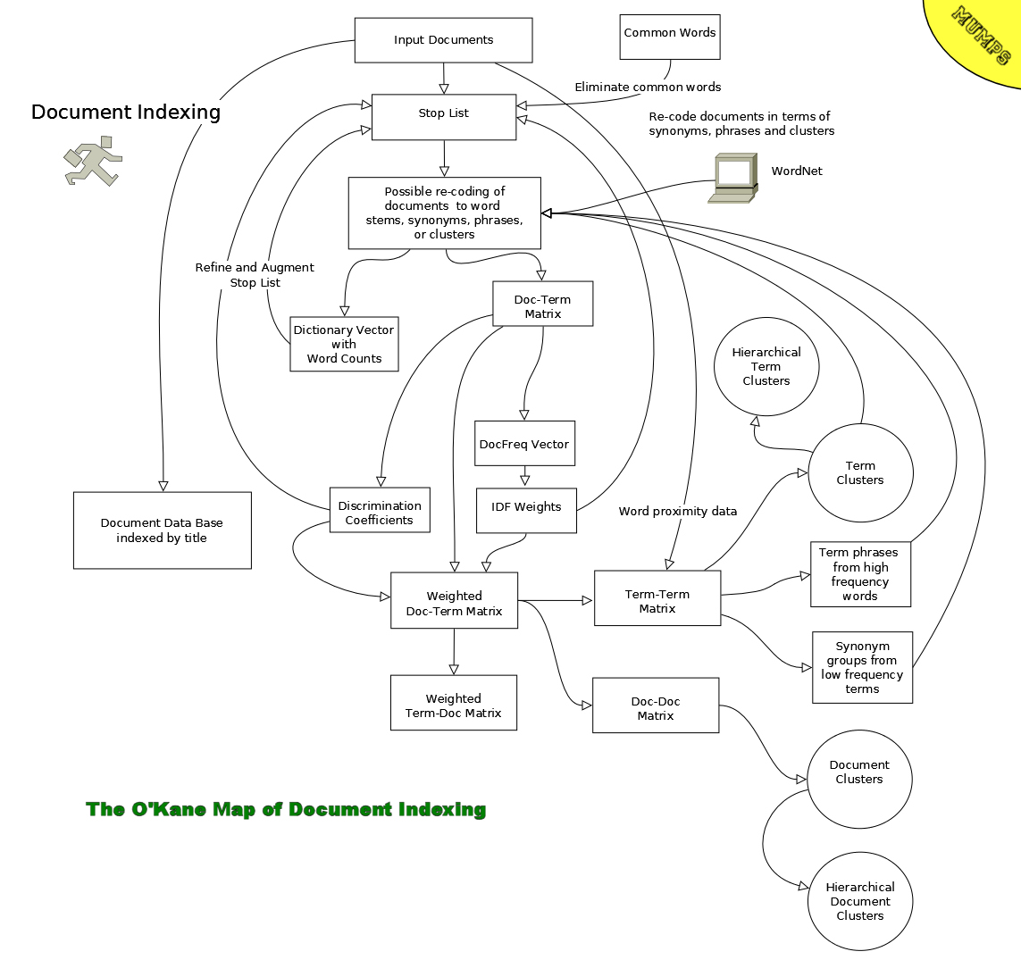
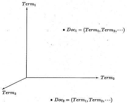
    One popular approach to automatic document indexing, the vector space model, views computer generated document vectors as describing a hyperspace in which the number of dimensions (axes) is equal to the number of indexing terms. This approach was originally proposed by G. Salton:

    Salton, G.; McGill, M.J., Introduction to Modern Information Retrieval, New York: McGraw Hill; 1983. Salton, G., The state of retrieval system evaluation, Information Processing & Management, 28(4): 441-449; 1992. Videos of a conference on Salton's work and on SMART are available at: The Open Video Project

    Each document vector is a point in that space defined by the distance along the axis associated with each document term proportional to the term's importance or significance in the document being represented. Queries are also portrayed as vectors that define points in the document hyperspace. Documents whose points in the hyperspace lie within an adjustable envelope of distance from the query vector point are retrieved. The information storage and retrieval process involves converting user typed queries to query vectors and correlating these with document vectors in order to select and rank documents for presentation to the user.

    Most (IR) systems have been implemented in C, Pascal and C++, although these languages provide little native support for the hyperspace model. Similarly, popular off-the-shelf legacy relational data base systems are inadequate to efficiently represent or manipulate sparse document vectors in the manner needed to effectively implement IR systems.

    

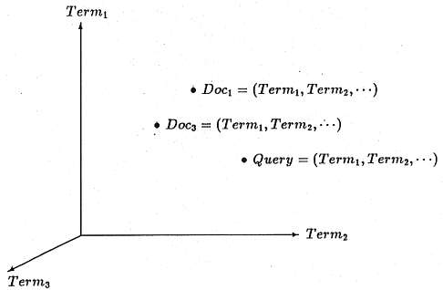
    Document are viewed as points in a hyperspace whose axes are the terms used in the document vectors. The location of a document in the space is determined by the degree to which the terms are present in a document. Some terms occur several times while other occur not at all. Terms also have weights associated with their content indicating strength and this is factored into the equation as well.

    

    Query vectors are also treated as points in the hyperspace and the documents that lie within a set distance of the query are determined to satisfy the query.

    

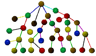
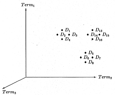
    Clustering involves identifying groupings of documents and constructing a cluster centroid vector to speed information storage and retrieval. Hierarchies of clusters can also be constructed.

    

    There are several formulae to calculate the distance between points in the hyperspace. One of the better known is the Cosine function illustrated in the figure above (from Salton 1983). In this formula, the Cosine between points is used to measure the distance. Some of the formulae are:

    

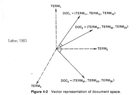
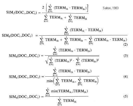
    In the above, taken from Salton 1983, the Cosine is formula 3. The formulae calculate the similarity between Doc_i and Doc_j by examining the relationships between term_i,k and term_j,k where term_i,k is the weight of term k in document i and term_j,k is the weight of term k in document j. Sim₁ is known as the Dice coefficient and Sim₂ is known as the Jaccard coefficient (see: Jaccard 1912, "The distribution of the flora of the alpine zone", New Phytologist 11:37-50).

    The following example illustrates the application of the above (from Salton 1983, pg 202-203):

    Doci = (3,2,1,0,0,0,1,1)
    Docj = (1,1,1,0,0,1,0,0)
    
    Sim1(Doci,Docj)= (2*6)/(8+4) -> 1
    Sim2(Doci,Docj)= (6)/(8+4-6) -> 1
    Sim3(Doci,Docj)= (6)/SQRT(16*4) -> 0.75 
    Sim4(Doci,Docj)= 6/4 ->  1.5
    Sim5(Doci,Docj)= 3/8 ->  0.375
    

11. Related Similarity Functions

    See Sam's String Metrics for a discussion of:

    1. Hamming distance
    2. Levenshtein distance
    3. Needleman-Wunch distance or Sellers Algorithm
    4. Smith-Waterman distance
    5. Gotoh Distance or Smith-Waterman-Gotoh distance
    6. Block distance or L1 distance or City block distance
    7. Monge Elkan distance
    8. Jaro distance metric
    9. Jaro Winkler
    10. SoundEx distance metric
    11. Matching Coefficient
    12. Dice.s Coefficient
    13. Jaccard Similarity or Jaccard Coefficient or Tanimoto coefficient
    14. Overlap Coefficient
    15. Euclidean distance or L2 distance
    16. Cosine similarity
    17. Variational distance
    18. Hellinger distance or Bhattacharyya distance
    19. Information Radius (Jensen-Shannon divergence)
    20. Harmonic Mean
    21. Skew divergence
    22. Confusion Probability
    23. Tau
    24. Fellegi and Sunters (SFS) metric
    25. TFIDF or TF/IDF
    26. FastA
    27. BlastP
    28. Maximal matches
    29. q-gram
    30. Ukkonen Algorithms

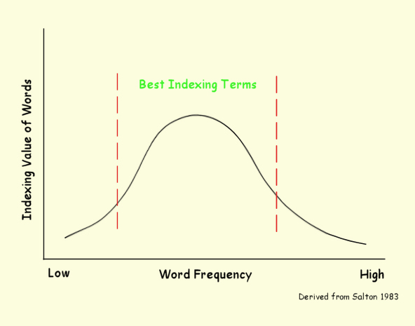
12. Assigning Word Weights

    Words used for indexing vary in their ability to indicate content and, thus, their importance as indexing terms. Some words, such as "the", "and", "was" and so forth are worthless as content indications and we eliminate them from consideration immediately. Other words occur so infrequently that they are also unlikely to be useful as indexing terms. Other words, however, with middle frequency of occurrence are candidates as indexing terms.

    However, not all words a equally good index terms. For example, the word "computer" in a collection of computer science articles conveys very little information useful to indexing the document since so many, if not all, the documents contain the word. The goal here is to determine a metric of the ability of a word to convey information.

    In the following example, several weighting schemes are compared. In the example, ^doc(i,w) is the number of times term w occurs in document i; ^dict(w) is the number of times term w occurs in the collection as a whole; ^df(w) is the number of documents term w occurs in; NbrDocs is the total number of documents in the collection; and the function $zlog() is the natural logarithm. The operation "\" is integer division.

    Normalize [normal.mps] Sun Dec 15 13:08:59 2002 1000 documents; 29942 word instances, 563 distinct words ^doc(i,w) Number times word w used in document i ^dict(w) Number times word w used in total collection ^df(w) Number of documents word w appears in Wgt1 ^doc(i,w)/(^dict(w)/^df(w)) Wgt2 ^doc(i,w)*$zlog(NbrDocs/^df(w))+1 Wgt3 Wgt1*Wgt2+0.5\1 Word ^doc(i,w) ^dict(w) ^df(w) Wgt1 Wgt2 Wgt3 MCA [1] Death of a cult. (Apple Computer needs to alter its strategy) (column) apple 4 261 112 1.716 9.757 17 -1.1625 computer 4 706 358 2.028 5.109 10 -19.4405 mac 2 146 71 0.973 6.290 6 -0.0256 macintosh 4 210 107 2.038 9.940 20 -0.5855 strategy 2 79 67 1.696 6.406 11 -0.0592 [2] Next year in Xanadu. (Ted Nelson's hypertext implementations) Swaine, - Michael. document 3 114 68 1.789 9.065 16 0.0054 operate 3 269 184 2.052 6.078 12 -2.1852 [3] WordPerfect. (WordPerfect for the Macintosh 2.0) (evaluation) Taub, Er- ic. edit 2 111 77 1.387 6.128 8 -0.0961 frame 2 9 7 1.556 10.924 17 0.0131 import 2 29 19 1.310 8.927 12 0.0998 macintosh 3 210 107 1.529 7.705 12 -0.5855 macro 3 38 24 1.895 12.189 23 0.1075 outstand 1 10 9 0.900 5.711 5 0.0168 user 4 861 435 2.021 4.330 9 -26.8094 wordperfect 8 24 8 2.667 39.627 106 0.1747 [4] Radius Pivot for Built-In Video an Radius Color Pivot. (Hardware Revie- w) (new Mac monitors)(includes related article on design of built-in 3 35 29 2.486 11.621 29 0.0678 color 3 81 47 1.741 10.173 18 0.0809 mac 2 146 71 0.973 6.290 6 -0.0256 monitor 6 88 52 3.545 18.739 66 0.0946 resolution 2 50 32 1.280 7.884 10 0.0288 screen 2 92 62 1.348 6.561 9 0.0199 video 4 106 61 2.302 12.188 28 0.0187 [5] CrystalPrint Express. (Software Review) (high-speed desktop laser prin- ter) (evaluation) desk 2 127 76 1.197 6.154 7 -0.1062 engine 1 15 13 0.867 5.343 5 0.0282 font 4 111 37 1.333 14.187 19 0.6350 laser 3 61 27 1.328 11.836 16 0.2562 print 3 140 66 1.414 9.154 13 0.0509 [6] 4D Write, 4D Calc, 4D XREF. (Software Review) (add-ins for Acius' Four- th Dimension database software) (evaluation) add-in 2 97 38 0.784 7.540 6 0.5551 analysis 2 179 139 1.553 4.947 8 -0.8492 database 5 138 67 2.428 14.515 35 0.1832 midrange 1 7 6 0.857 6.116 5 0.0218 spreadsheet 2 75 44 1.173 7.247 9 0.1707 vary 1 7 6 0.857 6.116 5 0.0107 [7] ConvertIt! (Software Review) (utility for converting HyperCard stacks - to IBM PC format) (evaluation) converter 2 24 13 1.083 9.686 10 0.0698 doe 5 97 84 4.330 13.385 58 -0.1139 graphical 2 307 171 1.114 4.532 5 -2.4079 hypercard 4 25 13 2.080 18.371 38 0.1517 mac 2 146 71 0.973 6.290 6 -0.0256 map 2 17 10 1.176 10.210 12 0.1180 program 4 670 334 1.994 5.386 11 -15.4832 script 3 54 32 1.778 11.326 20 0.1239 software 3 913 449 1.475 3.402 5 -30.7596 stack 5 15 8 2.667 25.142 67 0.0700 [8] Reports 2.0. (Software Review) (Nine To Five Software Reports 2.0 repo- rt generator for HyperCard 2.0) (evaluation) hypercard 5 25 13 2.600 22.714 59 0.1517 print 3 140 66 1.414 9.154 13 0.0509 software 3 913 449 1.475 3.402 5 -30.7596 stack 2 15 8 1.067 10.657 11 0.0700 [9] Project-scheduling tools. (FastTrack Schedule, MacSchedule) (Software - Review) (evaluation) manage 2 318 174 1.094 4.497 5 -2.4884 [10] Digital Darkroom. (Software Review) (new version of image-processing s- oftware) (evaluation) apply 1 17 15 0.882 5.200 5 0.0317 digital 4 90 52 2.311 12.826 30 -0.0042 image 4 107 58 2.168 12.389 27 0.1422 palette 2 18 12 1.333 9.846 13 0.0660 portion 2 17 15 1.765 9.399 17 0.0295 software 4 913 449 1.967 4.203 8 -30.7596 text 2 55 46 1.673 7.158 12 0.0304 user 5 861 435 2.526 5.162 13 -26.8094 [11] CalenDAr. (Software Review) (Psyborn Systems Inc. CalenDAr desk access- ory) (evaluation) accessory 2 14 10 1.429 10.210 15 0.0540 desk 2 127 76 1.197 6.154 7 -0.1062 display 2 106 78 1.472 6.102 9 -0.1278 program 3 670 334 1.496 4.290 6 -15.4832 sound 2 14 8 1.143 10.657 12 0.1172 user 3 861 435 1.516 3.497 5 -26.8094 [12] DisplayServer II-DPD. (Hardware Review) (DisplayServer II video card f- or using VGA monitor with Macintosh) (evaluation) apple 4 261 112 1.716 9.757 17 -1.1625 card 2 99 56 1.131 6.765 8 0.0790 display 2 106 78 1.472 6.102 9 -0.1278 macintosh 3 210 107 1.529 7.705 12 -0.5855 monitor 6 88 52 3.545 18.739 66 0.0946 vga 2 91 62 1.363 6.561 9 0.0104 video 2 106 61 1.151 6.594 8 0.0187 [13] SnapJot. (Software Review) (evaluation) Gruberman, Ken. capture 2 14 11 1.571 10.020 16 0.0271 image 3 107 58 1.626 9.542 16 0.1422 software 3 913 449 1.475 3.402 5 -30.7596 window 4 417 159 1.525 8.355 13 -3.4780 [14] Studio Vision. (Software Review) (Lehrman, Paul D.) (evaluation) Lehrm- an, Paul D. audio 1 8 6 0.750 6.116 5 0.0161 disk 3 234 121 1.551 7.336 11 -1.1468 edit 3 111 77 2.081 8.692 18 -0.0961 operate 2 269 184 1.368 4.386 6 -2.1852 portion 1 17 15 0.882 5.200 5 0.0295 requirement 2 87 76 1.747 6.154 11 -0.1203 sound 6 14 8 3.429 29.970 103 0.1172 user 3 861 435 1.516 3.497 5 -26.8094 [15] 70 things you need to know about System 7.0. (includes related article- s on past reports about System 7.0, Adobe Type 1 fonts, apple 3 261 112 1.287 7.568 10 -1.1625 communication 2 199 110 1.106 5.415 6 -0.6984 desk 2 127 76 1.197 6.154 7 -0.1062 disk 2 234 121 1.034 5.224 5 -1.1468 duplicate 1 10 9 0.900 5.711 5 0.0143 file 3 271 151 1.672 6.671 11 -1.3982 font 2 111 37 0.667 7.594 5 0.6350 memory 4 142 98 2.761 10.291 28 -0.2999 tip 1 8 6 0.750 6.116 5 0.0335 user 4 861 435 2.021 4.330 9 -26.8094 virtual 2 17 15 1.765 9.399 17 0.0424 [16] Data on the run. (Hardware Review) (palmtop organizers)(includes relat- ed article describing the WristMac from Microseeds character 2 25 17 1.360 9.149 12 0.0871 computer 4 706 358 2.028 5.109 10 -19.4405 data 3 415 226 1.634 5.462 9 -5.6011 database 2 138 67 0.971 6.406 6 0.1832 display 4 106 78 2.943 11.204 33 -0.1278 mac 3 146 71 1.459 8.935 13 -0.0256 ms_dos 2 98 65 1.327 6.467 9 0.0481 organize 1 19 17 0.895 5.075 5 0.0589 palmtop 1 6 5 0.833 6.298 5 0.0216 ram 2 145 93 1.283 5.750 7 -0.3992 review 2 265 238 1.796 3.871 7 -2.4234 rom 1 19 17 0.895 5.075 5 0.0374 software 4 913 449 1.967 4.203 8 -30.7596 transfer 2 66 44 1.333 7.247 10 0.0918 [17] High-speed, low-cost IIci cache cards. (includes related article on ca- ching for other Mac models) (buyers guide) cach 1 10 9 0.900 5.711 5 0.0127 cache 8 49 30 4.898 29.052 142 0.1613 card 6 99 56 3.394 18.294 62 0.0790 chip 2 117 67 1.145 6.406 7 -0.1153 high-speed 2 18 14 1.556 9.537 15 0.0352 memory 3 142 98 2.070 7.968 16 -0.2999 ram 2 145 93 1.283 5.750 7 -0.3992 [18] Mac, DOS and VAX file servers. (multiplatform file servers)(includes r- elated articles on optimizing server add-on 1 17 15 0.882 5.200 5 0.0374 apple 2 261 112 0.858 5.379 5 -1.1625 file 10 271 151 5.572 19.905 111 -1.3982 lan 2 98 51 1.041 6.952 7 0.0366 mac 4 146 71 1.945 11.580 23 -0.0256 macintosh 6 210 107 3.057 14.410 44 -0.5855 ms_dos 2 98 65 1.327 6.467 9 0.0481 netware 2 60 28 0.933 8.151 8 0.2314 network 6 571 222 2.333 10.030 23 -9.4287 ratio 1 18 16 0.889 5.135 5 0.0154 server 12 162 75 5.556 32.083 178 -0.1592 software 3 913 449 1.475 3.402 5 -30.7596 unix-based 1 15 13 0.867 5.343 5 0.0376 user 3 861 435 1.516 3.497 5 -26.8094 vax 2 28 14 1.000 9.537 10 0.1692 [19] Is it time for CD-ROM? (guide to 16 CD-ROM drives)(includes related ar- ticles on using IBM-compatible CD-ROMs with the Mac, audio 1 8 6 0.750 6.116 5 0.0161 cd-rom 9 31 13 3.774 40.085 151 0.1760 drive 9 249 129 4.663 19.431 91 -1.4872 macintosh 2 210 107 1.019 5.470 6 -0.5855 technology 2 335 220 1.313 4.028 5 -3.9304 [20] Silver platters that matter. (CD-ROM titles) (buyers guide) availe 3 135 121 2.689 7.336 20 -0.4302 cd-rom 6 31 13 2.516 27.057 68 0.1760 hypercard 2 25 13 1.040 9.686 10 0.1517 library 2 44 30 1.364 8.013 11 0.1473 macintosh 2 210 107 1.019 5.470 6 -0.5855

    In the example above, are document vectors for 20 documents (out of 1000) from computer science trade publications of the mid-80's are shown. Several weighting schemes are tried (see key at top). The MCA weight is the Modified Centroid Algorithm calculation method to calculate the Term Discrimination weight (see below).

13. Inverse Document Frequency and Basic Vector Space

    One of the simplest word weight schemes to implement is the Inverse Document Frequency weight. The IDF weight is the measure of how widely distributed a term is in a collection. Low IDF weights mean that the term is widely used while high weights indicate that the usage is more concentrated. The IDF weight measures the weight of a term in the collection as a whole, rather than the weight of a term in a document. In individual document vectors, the normalized frequency of occurrence of each term is multiplied by the IDF to give a weight for the term in the particular document. Thus, a term with a high frequency but a low IDF weight could still be a highly weighted term in a particular document, and, on the other hand, a term with a low frequency but a high IDF weight could also be an important term in a given document. The IDF weight for a term W in a collection of N documents is:

    

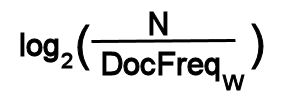
    where DocFreq_w is the number of documents in which term W occurs.

    1. OSU Medline Data Base IDF Weights

       The IDF weights for the OSU Medline collection were calculated after the words were processed by the stemming function $zstem() and the values are stored in the global array ^df(word) for subsequent use and also printed to standard output. The IDF weights for a recent run on the OSU data base is here: http://www.cs.uni.edu/~okane/source/ISR/medline.idf.sorted.gz. Note: due to tuning parameters that set thresholds for the construction of the stop list and other factors, different runs on the data base will produce some variation in the values displayed. The weights range from lows such as:

       0.189135 human
       0.288966 and
       0.300320 the
       0.542811 with
       0.737224 for
       0.793466 was
       0.867298 were
       

       to highs such as:

       12.590849 actinomycetoma
       12.590849 actinomycetomata
       12.590849 actinomycoma
       12.590849 actinomyosine
       12.590849 actinoplane
       12.590849 actinopterygii
       12.590849 actinoxanthin
       12.590849 actisomide
       12.590849 activ
       12.590849 activationin
       

       Note: for a given IDF value, the words are presented alphabetically. The OSU Medline collection has many code words that appear only once.

    2. Wikipedia Data Base IDF Weights

       Similarly, the Wikipedia IDF weights were calculated and the results are in http://www.cs.uni.edu/~okane/source/ISR/wiki.idf.sorted.gz. The weights range from lows such as:

       1.61 further
       1.62 either
       1.63 especial
       1.65 certain
       1.65 having
       1.67 almost
       1.67 along
       1.68 involve
       1.68 receive
       

       to highs such as:

       9.87 altopia
       9.87 alyque
       9.87 amangkur
       9.87 amarant
       9.87 amaranthus
       9.87 amarantine
       9.87 amazonite
       9.87 ambacht
       9.87 ambiorix
       

14. Calculating IDF Weights

    Calculating an IDF involves first building a document-term matrix (^doc(i,w)) where i is the document number and w is a term. Each cell in the document-term matrix will contain the count of the number of times that the term occurs in the document).

    Next, from the document-term matrix, construct a document frequency vector (^df(w)) where each element gives the number documents the term w occurs in.

    When the document frequency vector has been built, the individual IDF values for each word can be calculated.

    The following assumes you are using the file http://www.cs.uni.edu/~okane/source/ISR/medline.translated.txt.gz which is a pre-processed version of the OSU Medline text. The format of the file is:

    1. the code xxxxx115xxxxx followed by one blank
    2. the offset in the original text file of STAT- MEDLINE followed by a blank
    3. the document number followed by a blank
    4. one or more words, converted to lower case and stemmed by $zstem()

    Example:

    xxxxx115xxxxx 0 1 the bind acetaldehyde the active site ribonuclease alteration catalytic active ... xxxxx115xxxxx 2401 2 reduction breath ethanol reading norm male volunteer follow mouth rins with ... xxxxx115xxxxx 3479 3 does the blockade opioid receptor influence the development ethanol dependence ... xxxxx115xxxxx 4510 4 drinkwatcher description subject and evaluation laboratory marker heavy drink ... xxxxx115xxxxx 5745 5 platelet affinity for serotonin increased alcoholic and former alcoholic biological ... xxxxx115xxxxx 7128 6 clonidine alcohol withdraw pilot study differential symptom respons follow ... xxxxx115xxxxx 7915 7 bias survey drink habit this paper present data from genere populate survey ... xxxxx115xxxxx 8653 8 factor associate with young adult alcohol abuse the present study examne ... xxxxx115xxxxx 9862 9 alcohol and the elder relationship illness and smok group semi independent ... xxxxx115xxxxx 11174 10 concern the prob our confidence statistic editorial

    Calculating the IDF:

    Step 1

    1. delete any previous instances of the ^doc() and ^df() global arrays.

    Step 2

    Loop:

    1. Read the next word into w from the file using the $zzScan function.
    2. If $test is false, you have reached the end of file and proceed to Step 3.
    3. If the word w is the beginning of document token (xxxxx115xxxxx):
       1. read (use $zzScan) the offset and then the document number.
       2. Retain the document number as variable D.
       3. Store the offset at ^doc(D).
       4. Repeat the loop
    4. Check the word w against your stop list. If it is in the stop list, Repeat the loop
    5. If ^doc(D,w) exists, increment it; if not, create it with a value of 1.
    6. Repeat the loop

    Step 3

    1. for each document i in ^doc(i)
    2. for each word w in ^doc(i,w)
    3. check if ^df(w) exists. If it does, increment ^df(w); if not create ^df(w) and store a value of one.

    Step 4

    1. for each word in ^df(w)
    2. calculate its IDF using the value in ^df(w) (the number of documents the word occurs in) and D, the total number of documents.
    3. store the results in a global array ^idf(w)
    4. write (re-direct stdout is easiest) to a file the IDF value (2 decimal places are usually enough - see $justify), a blank, followed by the word.

    Step 5

    1. sort the file numerically according to IDF value (first field)

    The results of the IDF procedure may be used to enhance the stop list with words that have very low values.

    A basic program to create a document-term matrix and calculate IDF weights is:

    #!/usr/bin/mumps #+++++++++++++++++++++++++++++++++++++++++++++++++++++++++++++++++++ #+ #+ Mumps ISR Software Library #+ Copyright (C) 2006, 2008 by Kevin C. O'Kane #+ #+ Kevin C. O'Kane #+ okane@cs.uni.edu #+ #+ #+ This program is free software; you can redistribute it and/or modify #+ it under the terms of the GNU General Public License as published by #+ the Free Software Foundation; either version 2 of the License, or #+ (at your option) any later version. #+ #+ This program is distributed in the hope that it will be useful, #+ but WITHOUT ANY WARRANTY; without even the implied warranty of #+ MERCHANTABILITY or FITNESS FOR A PARTICULAR PURPOSE. See the #+ GNU General Public License for more details. #+ #+ You should have received a copy of the GNU General Public License #+ along with this program; if not, write to the Free Software #+ Foundation, Inc., 59 Temple Place, Suite 330, Boston, MA 02111-1307 USA #+ #++++++++++++++++++++++++++++++++++++++++++++++++++++++++++++++++++++++ # idf.mps February 22, 2008 kill ^df kill ^dict set %=$zStopInit("good") // loads stop list into a C++ container open 1:"translated.txt,old" if '$test write "translated not found",! halt use 1 for do . use 1 . set word=$zzScan . if '$test break . if word="xxxxx115xxxxx" set off=$zzScan,doc=$zzScan quit // new abstract . if '$zStopLookup(word) quit // is "word" in the good list . if $data(^doc(doc,word)) set ^doc(doc,word)=^doc(doc,word)+1 . else set ^doc(doc,word)=1 . if $data(^dict(word)) set ^dict(word)=^dict(word)+1 . else set ^dict(word)=1 use 5 close 1 set ^DocCount(1)=doc for d="":$order(^doc(d)):"" do . for w="":$order(^doc(d,w)):"" do .. if $data(^df(w)) set ^df(w)=^df(w)+1 .. else set ^df(w)=1 for w="":$order(^df(w)):"" do . set ^dfi(w)=$justify($zlog(doc/^df(w)),1,2) . write $justify(^dfi(w),1,2)," ",w,! write ! halt

    The program also records the offset in the original file of the beginning of the abstract and stores the IDF values in the vector ^dfi. It also calculates a document frequency vector (number of documents a term occurs in) ^df and a dictionary vector (total frequency of occurrence for each word) ^dict.

    Example results:

    http://www.cs.uni.edu/~okane/source/ISR/medline.idf.sorted.gz
    http://www.cs.uni.edu/~okane/source/ISR/medline.weighted-doc-vectors.gz
    http://www.cs.uni.edu/~okane/source/ISR/medline.weighted-term-vectors.gz

    http://www.cs.uni.edu/~okane/source/ISR/wiki.idf.sorted.gz
    http://www.cs.uni.edu/~okane/source/ISR/wiki.weighted-doc-vectors.gz
    http://www.cs.uni.edu/~okane/source/ISR/wiki.weighted-term-vectors.gz

15. Signal-noise ratio (see Salton83 links, pages 63-66)

16. Discrimination Coefficients (pages 66-71) and Simple Automatic Indexing (pages Salton83, 71-75); Willett 1985; Crouch 1988

    The Term Discrimination factor measures the degree to which a term differentiates one document from another. It is calculated based on the effect a term has on overall hyperspace density with and without a given term. If the space density is greater when a term is removed from consideration, that means the term was making documents look less like one another (a good discriminator) while terms whose remove decreases the density are poor discriminators. The discrimination values for a set of terms are similar to the values for the IDF weights but not exactly.

    The basic procedure calls for first calculating the average of pair-wise similarities between all documents in the space. Then for each word, the average of the pair-wise similarities of all the documents is calculated without that word. The difference in the averages is the term discrimination value for the word. When the average similarity increases when a word is removed, the word was a good discriminator - it made documents look less like one another. On the other hand, if the average similarity decreased, the term was not a good discriminator since it made the documents look more like one another. In practice, this is an expensive weight to calculate unless speed-up techniques are used.

    The modified centroid algorithm (see Crouch 1987), is an attempt to improve the speed of calculation. The exact calculation, where all pairwise similarity values are calculated each time, is of complexity of the order of (N)(N-1)(w)(W) where N is the number of documents, W is the number of words in the collection and w is the average number of terms per document vector.

    Crouch (1988) discusses several methods to speed this calculation. The first of these, the approximate approach, consists of calculating the similarities of the documents with a centroid vector representing the collection as a whole rather that pair-wise. This results in considerable simplification as the number of similarities to be calculated drops from (N)(N-1) to N.

    Another modification, called the Modified Centroid Algorithm is based on:

    • Subtracting the original contributions to the sum of the similarities of those documents containing some term W and replacing these values with the similarities calculated between the the centroid and the document vectors with W removed;
    • Storing the original contributions to the total similarity by each document in a vector for later use (rather than recalculating this value); and
    • Using an inverted list to identify those documents which contain the indexing terms.

    In the centroid approximation of discrimination coefficients, a centroid vector is calculated. That is, a vector is created whose individual components are the average usage of each word in the vocabulary. A centroid vector is the average of all the document vectors and, by analogy, is at the center of the hyperspace. When using a centroid vector, rather than calculating all the pair-wise similarities of each document with each other document, the average similarity is calculated by comparing each document with the centroid vector. This improves the performance to a complexity on the order of (N)(w)(W).

    As modified centroid algorithm (MCA) calculates the average similarity, it stores the contribution of each document to the total document density (order n space required). When calculating the effect of a term on the document space density, the MCA subtracts the original contribution of those documents that contain the term under consideration and re-adds the document's contribution re-calculated without the contribution of the term under consideration. Complexity is on the order of (DF)(w)(W) where DF is the average number of documents in which a term occurs. Finally, an inverted term-document matrix is used to quickly identify those documents that contain terms of interest rather than scanning through the entire document-term matrix looking for documents containing a given term.

    While the MCA method yields values that are only an approximation of the exact method, the values are very similar in most cases and the savings in time to calculate the coefficients is very significant. Crouch (Crouch 1987) reports that the MCA method was on the order of 527 times faster than the exact method on relatively small data sets. Larger data sets yield even greater savings as the time required for the exact method grows with the square of the number of documents while the MCA method grows linearly with the number of documents. The following is the basic MCA algorithm:

    #!/usr/bin/mumps #+++++++++++++++++++++++++++++++++++++++++++++++++++++++++++++++++++ #+ #+ Mumps ISR Software Library #+ Copyright (C) 2007, 2008 by Kevin C. O'Kane #+ #+ Kevin C. O'Kane #+ okane@cs.uni.edu #+ #+ #+ This program is free software; you can redistribute it and/or modify #+ it under the terms of the GNU General Public License as published by #+ the Free Software Foundation; either version 2 of the License, or #+ (at your option) any later version. #+ #+ This program is distributed in the hope that it will be useful, #+ but WITHOUT ANY WARRANTY; without even the implied warranty of #+ MERCHANTABILITY or FITNESS FOR A PARTICULAR PURPOSE. See the #+ GNU General Public License for more details. #+ #+ You should have received a copy of the GNU General Public License #+ along with this program; if not, write to the Free Software #+ Foundation, Inc., 59 Temple Place, Suite 330, Boston, MA 02111-1307 USA #+ #++++++++++++++++++++++++++++++++++++++++++++++++++++++++++++++++++++++ # discrim4.mps March 5, 2008 open 1:"discrim,new" use 1 set D=^DocCount(1) // number of documents kill ^mca set t1=$zd1 #++++++++++++++++++++++++++++++++++++++++++++++++++++++++++++++++++++++ # calculate centroid vector ^c() for entire collection and # the sum of the squares (needed in cos calc but should only be done once) #++++++++++++++++++++++++++++++++++++++++++++++++++++++++++++++++++++++ for w="":$order(^dict(w)):"" do . set ^c(w)=^dict(w)/D // centroid is composed of avg word usage #++++++++++++++++++++++++++++++++++++++++++++++++++++++++++++++++++++++ # Calculate total similarity of docs for all words (T) by # calculating the sum of the similarities of each document with the centroid. # Remember and store contribution of each document in ^dc(dn). #++++++++++++++++++++++++++++++++++++++++++++++++++++++++++++++++++++++ set T=0 for i="":$order(^doc(i)):"" do . set cos=$zzCosine(^doc(i),^c) . set ^dc(i)=cos // save contributions to total of each . set T=cos+T // sum the cosines #++++++++++++++++++++++++++++++++++++++++++++++++++++++++++++++++++++++ # calculate similarity of doc space with words removed #++++++++++++++++++++++++++++++++++++++++++++++++++++++++++++++++++++++ for W="":$order(^dict(W)):"" do // for each word W #++++++++++++++++++++++++++++++++++++++++++++++++++++++++++++++++++++++ # For each document containing W, calculate sum of the contribution # of the cosines of these documents to the total (T). ^dc(i) is # the original contribution of doc i. Sum of contributions is stored in T1. #++++++++++++++++++++++++++++++++++++++++++++++++++++++++++++++++++++++ . set T1=0,T2=0 . for d="":$order(^index(W,d)):"" do //for each doc d containing W .. set T1=^dc(d)+T1 // sum of orig contribution .. kill ^tmp .. for w1="":$order(^doc(d,w1)):"" do // make a copy of ^doc ... if w1=W quit // don't copy W ... set ^tmp(w1)=^doc(d,w1) .. set T2=T2+$zzCosine(^tmp,^c) // sum of cosines without W #++++++++++++++++++++++++++++++++++++++++++++++++++++++++++++++++++++++ # subtract original contribution with W (T1) and add contribution # without W (T2) and calculate r - the change, and store in ^mca(W) #++++++++++++++++++++++++++++++++++++++++++++++++++++++++++++++++++++++ # if old (T1) big and new (T2) small, density declines . set r=T2-T1*10000\1 . write r," ",^dfi(W)," ",W,! . set ^mca(W)=r use 5 write $zd1-t1,! close 1 halt

    The following is a further refinement of the above. It stores the sum of the squares of the components of the centroid vector which are needed in the denominator of each cosine calculation this eliminating this step This version also eliminates the step where a copy is made of the individual document vectors.

    Overall, the changes noted above and implemented in the program below can result in substantial time improvement. On a test run on 10,000 abstracts from the Medline database, the procedure above took 2,053 seconds while the one below took 378 seconds.

    #!/usr/bin/mumps #+++++++++++++++++++++++++++++++++++++++++++++++++++++++++++++++++++ #+ #+ Mumps ISR Software Library #+ Copyright (C) 2007, 2008 by Kevin C. O'Kane #+ #+ Kevin C. O'Kane #+ okane@cs.uni.edu #+ #+ #+ This program is free software; you can redistribute it and/or modify #+ it under the terms of the GNU General Public License as published by #+ the Free Software Foundation; either version 2 of the License, or #+ (at your option) any later version. #+ #+ This program is distributed in the hope that it will be useful, #+ but WITHOUT ANY WARRANTY; without even the implied warranty of #+ MERCHANTABILITY or FITNESS FOR A PARTICULAR PURPOSE. See the #+ GNU General Public License for more details. #+ #+ You should have received a copy of the GNU General Public License #+ along with this program; if not, write to the Free Software #+ Foundation, Inc., 59 Temple Place, Suite 330, Boston, MA 02111-1307 USA #+ #++++++++++++++++++++++++++++++++++++++++++++++++++++++++++++++++++++++ # discrim3.mps March 5, 2008 open 1:"discrim,new" use 1 set D=^DocCount(1) // number of documents set sq=0 kill ^mca set t1=$zd1 #++++++++++++++++++++++++++++++++++++++++++++++++++++++++++++++++++++++ # calculate centroid vector ^c() for entire collection and # the sum of the squares (needed in cos calc but should only be done once) #++++++++++++++++++++++++++++++++++++++++++++++++++++++++++++++++++++++ for w="":$order(^dict(w)):"" do . set ^c(w)=^dict(w)/D // centroid is composed of avg word usage . set sq=^c(w)**2+sq // The sum of the squares is needed below. #++++++++++++++++++++++++++++++++++++++++++++++++++++++++++++++++++++++ # Calculate total similarity of doc for all words (T) space by # calculating the sum of the similarities of each document with the centroid. # Remember and store contribution of each document in ^dc(dn). #++++++++++++++++++++++++++++++++++++++++++++++++++++++++++++++++++++++ set T=0 for i="":$order(^doc(i)):"" do . set x=0 . set y=0 . for w="":$order(^doc(i,w)):"" do .. set d=^doc(i,w) .. set x=d*^c(w)+x // numerator of cos(c,doc) calc .. set y=d*d+y // part of denominator #++++++++++++++++++++++++++++++++++++++++++++++++++++++++++++++++++++++ # Calculate and store the cos(c,doc(i)). # Remember in ^dc(i) the contribution that this document made to the total. #++++++++++++++++++++++++++++++++++++++++++++++++++++++++++++++++++++++ . if y=0 quit . set ^dc(i)=x/$zroot(sq*y) // cos(c,doc(i)) . set T=^dc(i)+T // sum the cosines #++++++++++++++++++++++++++++++++++++++++++++++++++++++++++++++++++++++ # calculate similarity of doc space with words removed #++++++++++++++++++++++++++++++++++++++++++++++++++++++++++++++++++++++ for W="":$order(^dict(W)):"" do #++++++++++++++++++++++++++++++++++++++++++++++++++++++++++++++++++++++ # For each document containing W, calculate sum of the contribution # of the cosines of these documents to the total (T). ^dc(i) is # the original contribution of doc i. Sum of contributions is stored in T1. #++++++++++++++++++++++++++++++++++++++++++++++++++++++++++++++++++++++ . set T1=0,T2=0 . for i="":$order(^index(W,i)):"" do // row of doc nbrs for word .. set T1=^dc(i)+T1 // use prevsly calc'd cos #++++++++++++++++++++++++++++++++++++++++++++++++++++++++++++++++++++++ # For each word in document i, recalculate cos(c,doc) but without word W #++++++++++++++++++++++++++++++++++++++++++++++++++++++++++++++++++++++ .. set x=0 .. set y=0 .. for w="":$order(^doc(i,w)):"" do ... if w'=W do // if W not w .... set d=^doc(i,w) .... set x=d*^c(w)+x // d*^c(w)+x .... set y=d**2+y .. if y=0 quit .. set T2=x/$zr(sq*y)+T2 // T2 sums cosines without W #++++++++++++++++++++++++++++++++++++++++++++++++++++++++++++++++++++++ # subtract original contribution with W (T1) and add contribution # without W (T2) and calculate r - the change, and store in ^mca(W) #++++++++++++++++++++++++++++++++++++++++++++++++++++++++++++++++++++++ # if old (T1) big and new (T2) small, density declines . set r=T2-T1*10000\1 . write r," ",^dfi(W)," ",W,! . set ^mca(W)=r use 5 write "Time used: ",$zd1-t1,! close 1 halt

    Example results:

    wiki.discrim.gz .
    medline.discrim.sorted.gz .

    Note: the discrimination coefficients output is in three columns: the first is the coefficient times 10,000, the second is the IDF for the word and the third is the word.

17. Basic Retrieval

18. Scanning the doc-term matrix

    A simple program to scan the document-term matrix looking for documents that have terms from a query vector. (Results based on 20,000 documents).

    #!/usr/bin/mumps # tq.mps Feb 27, 2008 kill ^query write "Enter search terms: " read a if a="" halt for i=1:1 do . set b=$piece(a," ",i) . if b="" break . set b=$zn(b) // lower case, no punct . set b=$zstem(b) // stem it . set ^query(b)="" if $order(^query(""))="" halt for j="":$order(^query(j)):"" write j,! set t1=$zd1 for i="":$order(^doc(i)):"" do . set f=1 . for j="":$order(^query(j)):"" do .. if '$d(^doc(i,j)) set f=0 break . if f write i,?8,$extract(^t(i),1,70),! write !,"Elapsed time: ",$zd1-t1,! Enter search terms: epithelial fibrosis epithelial fibrosis 10001 Phosphorylation fails to activate chloride channels from cystic fibro 18197 Relationship between mammographic and histologic features of breast t 6944 Cyclic adenosine monophosphate-dependent kinase in cystic fibrosis tr Elapsed time: 1

19. Scanning the term-doc matrix

    A simple program to scan the term-document matrix looking for documents that contain a search term.

    #!/usr/bin/mumps #+++++++++++++++++++++++++++++++++++++++++++++++++++++++++++++++++++ #+ #+ Mumps ISR Software Library #+ Copyright (C) 2008 by Kevin C. O'Kane #+ #+ Kevin C. O'Kane #+ okane@cs.uni.edu #+ #+ #+ This program is free software; you can redistribute it and/or modify #+ it under the terms of the GNU General Public License as published by #+ the Free Software Foundation; either version 2 of the License, or #+ (at your option) any later version. #+ #+ This program is distributed in the hope that it will be useful, #+ but WITHOUT ANY WARRANTY; without even the implied warranty of #+ MERCHANTABILITY or FITNESS FOR A PARTICULAR PURPOSE. See the #+ GNU General Public License for more details. #+ #+ You should have received a copy of the GNU General Public License #+ along with this program; if not, write to the Free Software #+ Foundation, Inc., 59 Temple Place, Suite 330, Boston, MA 02111-1307 USA #+ #++++++++++++++++++++++++++++++++++++++++++++++++++++++++++++++++++++++ # tqw.mps Feb 28, 2008 kill ^query kill ^tmp write "Enter search terms: " read a if a="" halt for i=1:1 do . set b=$piece(a," ",i) . if b="" break . set b=$zn(b) // lower case, no punct . set b=$zstem(b) // stem it . set ^query(b)=1 if $order(^query(""))="" halt set q=0 for w="":$order(^query(w)):"" write w," " set q=q+1 write ! set t1=$zd1 for w="":$order(^query(w)):"" do . for i="":$order(^index(w,i)):"" do .. if $data(^tmp(i)) set ^tmp(i)=^tmp(i)+1 .. else set ^tmp(i)=1 for i="":$order(^tmp(i)):"" do . if ^tmp(i)=q write i,?8,$j($zzCosine(^doc(i),^query),5,3)," ",$extract(^t(i),1,70),! write !,"Elapsed time: ",$zd1-t1,! Enter search terms: epithelial fibrosis 10001 0.180 Phosphorylation fails to activate chloride channels from cystic fibro 18197 0.291 Relationship between mammographic and histologic features of breast t 6944 0.323 Cyclic adenosine monophosphate-dependent kinase in cystic fibrosis tr Elapsed time: 0

20. Weighted scanning the term-doc matrix

    Similar to the above but all terms not required. Results sorted by sum of weights of terms in the documents.

    Note: the $job function returns the process id of the running program. This is unique and it is used to name a temporary file that contains the unsorted results.

    #!/usr/bin/mumps # tqw1.mps Feb 27, 2008 kill ^query kill ^tmp write "Enter search terms: " read a if a="" halt for i=1:1 do . set b=$piece(a," ",i) . if b="" break . set b=$zn(b) // lower case, no punct . set b=$zstem(b) // stem it . set ^query(b)="" if $order(^query(""))="" halt set q=0 for w="":$order(^query(w)):"" write w," " set q=q+1 write ! set t1=$zd1 for w="":$order(^query(w)):"" do . for i="":$order(^index(w,i)):"" do .. if $data(^tmp(i)) set ^tmp(i)=^tmp(i)+^index(w,i) .. else set ^tmp(i)=^index(w,i) set fn=$job_",new" open 1:fn // $job number is unique to this process use 1 for i="":$order(^tmp(i)):"" do . write ^tmp(i)," ",$extract(^t(i),1,70),! close 1 use 5 set %=$zsystem("sort -n "_$job_"; rm "_$job) write !,"Elapsed time: ",$zd1-t1,! Enter search terms: epithelial fibrosis epithelial fibrosis 9.02 Adaptation of the jejunal mucosa in the experimental blind loop syndr 9.02 Adherence of Staphylococcus aureus to squamous epithelium: role of fi 9.02 Anti-Fx1A induces association of Heymann nephritis antigens with micr 9.02 Anti-human tumor antibodies induced in mice and rabbits by "internal 9.02 Bacterial adherence: the attachment of group A streptococci to mucosa 9.02 Benign persistent asymptomatic proteinuria with incomplete foot proce 9.02 Binding of navy bean (Phaseolus vulgaris) lectin to the intestinal ce 9.02 Cellular and non-cellular compositions of crescents in human glomerul 9.02 Central nervous system metastases in epithelial ovarian carcinoma. ... 27.06 A new model system for studying androgen-induced growth and morphogen 27.06 Immunohistochemical observations on binding of monoclonal antibody to 27.7 Cyclic adenosine monophosphate-dependent kinase in cystic fibrosis tr 28.34 Relationship between mammographic and histologic features of breast t 28.98 Asbestos induced diffuse pleural fibrosis: pathology and mineralogy. 28.98 High dose continuous infusion of bleomycin in mice: a new model for d 28.98 Taurine improves the absorption of a fat meal in patients with cystic 33.81 Measurement of nasal potential difference in adult cystic fibrosis, Y 43.47 Are lymphocyte beta-adrenoceptors altered in patients with cystic fib 43.47 Lipid composition of milk from mothers with cystic fibrosis. 57.96 Pulmonary abnormalities in obligate heterozygotes for cystic fibrosis Elapsed time: 0

21. Scripted test runs

    Often it is better to break the indexing process into multiple steps. The Mumps interpreter generally runs faster when the run-time symbol table is not cluttered with many variable names. Also, using a script can provide an easy way to set parameters to the several steps from one central code point.

    Below is the bash script used to do the test runs in this book. It invokes many individual Mumps programs as well as other system resources such as sort.

    The script generally takes a considerable amount of time to execute so it is often run under the control of nohup. This permits the user to logoff and the script to continue running. All output generated during execution that would otherwise appear on your screed (stdout and stderr) will instead be captured and written to the file nohup.out.

    To invoke a script with nohup type:

          nohup nice scriptName &
    

    nohup will initiate the script and capture the output. The nice command causes your script to run at a slightly reduced priority thus giving interactive users preference. The & causes the processes to run in the background thus giving you a command prompt immediately (rather than when the script is complete). Note: is you want to kill the script, type ps and then kill -9 pid where pid is the process id of the script. You may also want to kill the program currently running as killing the script only stops the starting of additional tasks; tasks in execution continue in execution.

    Note that the Mumps interpreter always looks for QUERY_STRING in the environment. Thus, if you create QUERY_STRING and place in it parameters, Mumps will read these and create variables with values as is the case when your program is invoked by the web server:

          QUERY_STRING="idf=$TT_MIN_IDF&cos=$TT_MIN_COS"
          export QUERY_STRING
    

    In the example above, query string is build and exported to the environment. It contains two assignment clauses that will result in the variables idf and cos being created and initialized in Mumps before your program begins execution. the bash variables TT_MIN_IDF and TT_MIN_COS are established at the beginning of the script and their values are substituted when QUERY_STRING is created. Note the $'s - these cause the substitution and are required by bash syntax.

    #!/bin/bash #+++++++++++++++++++++++++++++++++++++++++++++++++++++++++++++++++++ #+ #+ Mumps Information Storage and Retrieval Software Library #+ Copyright (C) 2006, 2008 by Kevin C. O'Kane #+ #+ Kevin C. O'Kane #+ okane@cs.uni.edu #+ #+ #+ This program is free software; you can redistribute it and/or modify #+ it under the terms of the GNU General Public License as published by #+ the Free Software Foundation; either version 2 of the License, or #+ (at your option) any later version. #+ #+ This program is distributed in the hope that it will be useful, #+ but WITHOUT ANY WARRANTY; without even the implied warranty of #+ MERCHANTABILITY or FITNESS FOR A PARTICULAR PURPOSE. See the #+ GNU General Public License for more details. #+ #+ You should have received a copy of the GNU General Public License #+ along with this program; if not, write to the Free Software #+ Foundation, Inc., 59 Temple Place, Suite 330, Boston, MA 02111-1307 USA #+ #++++++++++++++++++++++++++++++++++++++++++++++++++++++++++++++++++++++ # clear old nohup.out cat /dev/null > nohup.out # medline MedlineInterp.script March 9, 2008 TRUE=1 FALSE=0 # maximum number of documents to scan MAX_DOCS=20000 # maximum word occurrence for stopselect.mps MAX_WORDS=1000 # minumum word occurrence for stopselect.mps MIN_WORDS=5 # minimum IDF value for doc-doc matrix DD_MIN_IDF=7 # minimum DD cosine weight DD_MIN_WGT=0.8 # minimum weight in weight.mps MIN_WEIGHT=5 # minimum IDF in tt.mps TT_MIN_IDF=5 # minimum IDF cosine TT_MIN_COS=0.8 # minimum co-occurence tt count TT_MIN_COUNT=10 # perform steps: DO_ZIPF=$TRUE DO_TT=$TRUE DO_CONVERT=$TRUE DO_DICTIONARY=$TRUE DO_STOPSELECT=$TRUE DO_IDF=$TRUE DO_WEIGHT=$TRUE DO_COHESION=$TRUE DO_JACCARD=$TRUE DO_TTCLUSTER=$TRUE DO_DISCRIM=$TRUE DO_DOCDOC=$TRUE DO_CLUSTERS=$TRUE DO_HIERARCHY=$TRUE DO_TEST=$TRUE if [ $DO_COHESION -eq $TRUE ] then DO_TT=$TRUE fi if [ $DO_JACCARD -eq $TRUE ] then DO_TT=$TRUE fi # delete any prior data bases rm key.dat rm data.dat if [ $DO_CONVERT -eq $TRUE ] then echo "Convert data base format" date starttime.mps QUERY_STRING="MAX=$MAX_DOCS" export QUERY_STRING echo "MAX documents to read $QUERY_STRING" reformat.mps < osu.medline > rtrans.txt stems.mps < rtrans.txt > translated.txt echo "Conversion done - total time: `endtime.mps`" echo fi if [ $DO_DICTIONARY -eq $TRUE ] then echo "Generate and sort word frequency list" date starttime.mps dictionary.mps < translated.txt > dictionary.unsorted sort -nr < dictionary.unsorted > dictionary.sorted echo "Word frequency list done - total time: `endtime.mps`" echo fi if [ $DO_ZIPF -eq $TRUE ] then echo "Zipf calculation" date starttime.mps Zdictionary.mps < rtrans.txt | sort -nr | zipf.mps > medline.zipf endtime.mps echo fi echo "Count documents" grep "xxxxx115" translated.txt | wc > DocStats echo "Document grep result:" cat DocStats if [ $DO_STOPSELECT -eq $TRUE ] then echo "Select good words" date starttime.mps QUERY_STRING="max=$MAX_WORDS&min=$MIN_WORDS" export QUERY_STRING echo "QUERY_STRING = $QUERY_STRING" ls -l dictionary.sorted stopselect.mps < dictionary.sorted > good echo "Good word selection time: `endtime.mps`" rm dictionary.unsorted echo fi if [ $DO_IDF -eq $TRUE ] then echo "Generate and sort IDF weights" date starttime.mps idf.mps > idf.unsorted echo "idf done" sort -n < idf.unsorted > idf.sorted echo "IDF time: `endtime.mps`" rm idf.unsorted fi if [ $DO_WEIGHT -eq $TRUE ] then echo "Create weighted doc vectors" date starttime.mps # set minimum IDF*Freq value QUERY_STRING="idfmin=$MIN_WEIGHT" export QUERY_STRING echo "QUERY_STRING = $QUERY_STRING" weight.mps echo "Weighting time: `endtime.mps`" echo fi echo "Dump/restore" echo "Old data base sizes:" ls -lh key.dat data.dat QUERY_STRING="file=weight.dmp" export QUERY_STRING starttime.mps dump.mps rm key.dat rm data.dat restore.mps echo "New data base sizes:" ls -lh key.dat data.dat echo "Dump/restore time: `endtime.mps`" echo if [ $DO_TT -eq $TRUE ] then echo "Calculate and sort term-term matrix" date QUERY_STRING="min=$TT_MIN_COUNT&idf=$TT_MIN_IDF&cos=$TT_MIN_COS" export QUERY_STRING starttime.mps tt.mps > tt sort -n < tt > tt.sorted echo "Term-term time: `endtime.mps`" echo if [ $DO_COHESION -eq $TRUE ] then echo "Calculate and sort cohesion matrix" date starttime.mps cohesion.mps > cohesion sort -nr < cohesion > cohesion.sorted echo "Cohesion time: `endtime.mps`" echo fi if [ $DO_JACCARD -eq $TRUE ] then echo "Calculate and sort jaccard term-term matrix" date starttime.mps jaccard-tt.mps > jaccard-tt sort -n < jaccard-tt > jaccard-tt.sorted echo "Jaccard term time: `endtime.mps`" echo fi if [ $DO_TTCLUSTER -eq $TRUE ] then echo "Calculate term clusters" date starttime.mps clustertt.mps > cluster-tt echo "Cluster term time: `endtime.mps`" echo fi fi if [ $DO_DISCRIM -eq $TRUE ] then echo "Calculate discrimination co-efficients" date starttime.mps discrim3.mps echo "discrim.mps time: `endtime.mps`" sort -n < discrim > discrim.sorted echo fi echo "Dump/restore" date echo "Old data base size:" ls -lh key.dat data.dat QUERY_STRING="file=discrim.dmp" export QUERY_STRING starttime.mps dump.mps rm key.dat rm data.dat restore.mps echo "New data base size:" ls -lh key.dat data.dat echo "dump/restore end: `endtime.mps`" echo if [ $DO_DOCDOC -eq $TRUE ] then echo "Calculate document-document matrix" date starttime.mps QUERY_STRING="wgt=$DD_MIN_WGT&min=$DD_MIN_IDF" export QUERY_STRING echo "QUERY_STRING = $QUERY_STRING" docdoc5.mps > dd2 echo "Doc-doc time: `endtime.mps`" echo fi if [ $DO_CLUSTERS -eq $TRUE ] then echo "Calculate clusters" date starttime.mps cluster1.mps > clusters echo "Cluster time: `endtime.mps`" echo fi if [ $DO_HIERARCHY -eq $TRUE ] then echo "Calculate hierarchy" date starttime.mps ttfolder.mps > ttfolder echo "Hierarchy time: `endtime.mps`" echo echo "Calculate tables" date starttime.mps tab.mps < ttfolder > tab index.mps echo "Hierarchy time: `endtime.mps`" echo fi if [ $DO_TEST -eq $TRUE ] then echo "alcohol" > tstquery echo "test query is alcohol" medlineRetrieve.mps < tstquery fi

22. Simple Retrieval

    The following program reads in a set of query words into a query vector and then calculates the cosines between the query and the document vectors. It then prints out the titles of the 10 documents with the highest cosine correlations with the query. Note: this program makes use of a synonym dictionary which will be discussed below.

    Basic Retrieval

    #!/usr/bin/mumps #+++++++++++++++++++++++++++++++++++++++++++++++++++++++++++++++++++ #+ #+ Mumps ISR Software Library #+ Copyright (C) 2005, 2007, 2008 by Kevin C. O'Kane #+ #+ Kevin C. O'Kane #+ okane@cs.uni.edu #+ #+ #+ This program is free software; you can redistribute it and/or modify #+ it under the terms of the GNU General Public License as published by #+ the Free Software Foundation; either version 2 of the License, or #+ (at your option) any later version. #+ #+ This program is distributed in the hope that it will be useful, #+ but WITHOUT ANY WARRANTY; without even the implied warranty of #+ MERCHANTABILITY or FITNESS FOR A PARTICULAR PURPOSE. See the #+ GNU General Public License for more details. #+ #+ You should have received a copy of the GNU General Public License #+ along with this program; if not, write to the Free Software #+ Foundation, Inc., 59 Temple Place, Suite 330, Boston, MA 02111-1307 USA #+ #++++++++++++++++++++++++++++++++++++++++++++++++++++++++++++++++++++++ # simpleRetrieval.mps Feb 28, 2008 open 1:"osu.medline,old" if '$test write "osu.medline not found",! halt write "Enter query: " kill ^query kill ^ans for do // extract query words to query vector . set w=$zzScanAlnum . if '$test break . set w=$zstem(w) . set ^query(w)=1 write "Query is: " for w="":$order(^query(w)):"" write w," " write ! set time0=$zd1 for i="":$order(^doc(i)):"" do // calculate cosine between query and each doc . if i="" break . set c=$zzCosine(^doc(i),^query) # If cosine is > zero, put it and the doc offset (^doc(i)) into an answer vector. # Make the cosine a right justified string of length 5 with 3 digits to the # right of the decimal point. This will force numeric ordering on the first key. . if c>0 set ^ans($justify(c,5,3),^doc(i))="" write "results:",! set x="" for %%=1:1:10 do . set x=$order(^ans(x),-1) // cycle thru cosines in reverse (descending) order. . if x="" break . for i="":$order(^ans(x,i)):"" do .. use 1 set %=$zseek(i) // move to correct spot in file primates.text .. read a // skip STAT- MEDLINE .. for k=1:1:30 do // the limit of 30 is to prevent run aways. ... use 1 ... read a // find the title ... if $extract(a,1,3)="TI " use 5 write x," ",$extract(a,7,80),! ... if $extract(a,1,3)="AB " for do .... use 5 .... write ?5,$extract(a,7,120),! .... use 1 .... read a .... if '$test break .... if $extract(a,1,3)'=" " break ... if $extract(a,1,3)="STA" use 5 write ! break write !,"Time used: ",$zd1-time0," seconds",! which produces the following results on the first 20,000 abstracts: Enter query: epithelial fibrosis Query is: epithelial fibrosis results: 0.393 Epithelial tumors of the ovary in women less than 40 years old. From Jan 1, 1978 through Dec 31, 1983, 64 patients with epithelial ovarian tumors, frankly malignant or borderline, were managed at one institution. Nineteen patients (29.7%) were under age 40. The youngest patient was 19 years old. Nulliparity was present in 32% of this group of patients. Of these young patients, 58% had borderline epithelial tumors, compared to 13% of patients over 40 years of age. Twenty-one percent of the young patients were initially managed by unilateral adnexal surgery. The overall cumulative actuarial survival rate of all young patients was 93%. Young patients with epithelial ovarian tumors tend to have earlier grades of epithelial neoplasms, and survival is better than that reported for older patients with similar tumors. 0.367 Misdiagnosis of cystic fibrosis. On reassessment of 179 children who had previously been diagnosed as having cystic fibrosis seven (4%) were found not to have the disease. The importance of an accurate sweat test is emphasised as is the necessity to prove malabsorption or pancreatic abnormality to support the diagnosis of cystic fibrosis. 0.367 Are lymphocyte beta-adrenoceptors altered in patients with cystic fibrosis 1. Beta-adrenergic responsiveness may be decreased in cystic fibrosis. In order to determine whether this reflects an alteration in the human lymphocyte beta-receptor complex, we studied 12 subjects with cystic fibrosis (six were stable and ambulatory and six were decompensated, hospitalized) as compared with 12 normal controls. 2. Lymphocyte beta-receptor mediated adenylate cyclase activity (EC 4.6.1.1) was not decreased in the ambulatory cystic fibrosis patients as compared with controls. In contrast, decompensated hospitalized cystic fibrosis patients demonstrated a significant reduction in beta-receptor mediated lymphocyte adenylate cyclase activity expressed as the relative increase over basal levels stimulated by the beta-agonist isoprenaline compared with both normal controls and stable ambulatory cystic fibrosis patients (control 58 +/- 4%; ambulatory cystic fibrosis patients 51 +/- 7%; decompensated hospitalized cystic fibrosis patients 28 +/- 5%; P less than 0.05). 3. Our data suggest that defects in lymphocyte beta-receptor properties in cystic fibrosis patients may be better correlated with clinical status than with presence or absence of the disease state. 0.352 Measurement of nasal potential difference in adult cystic fibrosis, Young' Previous work confirmed the abnormal potential difference between the undersurface of the inferior nasal turbinate and a reference electrode in cystic fibrosis, but the technique is difficult and the results show overlap between the cystic fibrosis and the control populations. In the present study the potential difference from the floor of the nose has therefore been assessed in normal subjects, as well as in adult patients with cystic fibrosis, bronchiectasis and Young's syndrome. Voltages existing along the floor of the nasal cavity were recorded. The mean potential difference was similar in controls (-18 (SD 5) mv) and in patients with bronchiectasis (-17 (6) mv) and Young's syndrome (-20 (6) mv). The potential difference in cystic fibrosis (-45 (8) mv) was significantly different from controls (p less than 0.002) and there was no overlap between the cystic fibrosis values and values obtained in normal and diseased controls. This simple technique therefore discriminates well between patients with cystic fibrosis and other populations, raising the possibility of its use to assist in diagnosis. 0.342 Pulmonary abnormalities in obligate heterozygotes for cystic fibrosis. Parents of children with cystic fibrosis have been reported to have a high prevalence of increased airway reactivity, but these studies were done in a select young, healthy, symptomless population. In the present study respiratory symptoms were examined in 315 unselected parents of children with cystic fibrosis and 162 parents of children with congenital heart disease (controls). The cardinal symptom of airway reactivity, wheezing, was somewhat more prevalent in cystic fibrosis parents than in controls, but for most subgroups this increased prevalence did not reach statistical significance. Among those who had never smoked, 38% of obligate heterozygotes for cystic fibrosis but only 25% of the controls reported wheezing (p less than 0.05). The cystic fibrosis parents who had never smoked but reported wheezing had lower FEV1 and FEF25-75, expressed as a percentage of the predicted value, than control parents; and an appreciable portion of the variance in pulmonary function was contributed by the interaction of heterozygosity for cystic fibrosis with wheezing. For cystic fibrosis parents, but not controls, the complaint of wheezing significantly contributed to the prediction of pulmonary function (FEV1 and FEF25-75). In addition, parents of children with cystic fibrosis reported having lung disease before the age of 16 more than twice as frequently as control parents. Other respiratory complaints, including dyspnoea, cough, bronchitis, and hay fever, were as common in controls as in cystic fibrosis heterozygotes. These data are consistent with the hypothesis that heterozygosity for cystic fibrosis is associated with increased airway reactivity and its symptoms, and that the cystic fibrosis heterozygotes who manifest airway reactivity and its symptoms may be at risk for poor pulmonary function. 0.323 Retroperitoneal fibrosis and nonmalignant ileal carcinoid. The carcinoid syndrome and fibrosis are unusual but identifiable disease processes. We report a rare case of retroperitoneal fibrosis associated with an ileal carcinoid in the absence of metastatic disease. The literature is reviewed. 0.323 Cyclic adenosine monophosphate-dependent kinase in cystic fibrosis trachea Cl-impermeability in cystic fibrosis (CF) tracheal epithelium derives from a deficiency in the beta-adrenergic regulation of apical membrane Cl- channels. To test the possibility that cAMP-dependent kinase is the cause of this deficiency, we assayed this kinase in soluble fractions from cultured airway epithelial cells, including CF human tracheal epithelial cells. Varying levels of cAMP were used in these assays to derive both a Vmax and apparent dissociation constant (Kd) for the enzymes in soluble extracts. The cAMP-dependent protein kinase from CF human tracheal epithelial cells has essentially the same Vmax and apparent Kd as non-CF human, bovine, and dog tracheal epithelial cells. Thus, the total activity of the cAMP-dependent kinases and their overall responsiveness to cAMP are unchanged in CF. 0.313 Poor prognosis in patients with rheumatoid arthritis hospitalized for inte Fifty-seven patients with rheumatoid arthritis (RA) were treated in hospital for diffuse interstitial lung fibrosis. Although interstitial fibrosis (either on the basis of lung function tests or chest roentgenograms or both) is fairly common among patients with RA, according to this study interstitial fibrosis of sufficient extent or severity to warrant hospitalization was rare: incidence of hospitalization due to the lung disease in RA patients was one case per 3,500 patient-years. Eight patients had a largely reversible lung disease associated with drug treatment (gold, D-penicillamine or nitrofurantoin.) The remaining 49 had interstitial fibrosis of unknown cause. Causes for hospitalization were respiratory and general symptoms in 38, but infiltrations on routine chest roentgenographic examinations alone in eleven patients. Forty-five out of the 49 patients had crackles on auscultation. The most typical findings in lung function tests were restriction and a decreased diffusion capacity. These 49 patients showed a poor prognosis, with a median survival of 3.5 years and a five-year survival rate of 39 percent. 0.291 Relationship between mammographic and histologic features of breast tissue Mammograms and histologic slides of a group of 320 women who had breast symptoms and a biopsy without cancer being found were reviewed. The mammographic features assessed were the parenchymal pattern and extent of nodular and homogeneous densities. In addition to the pathologic diagnosis, the histologic features assessed included epithelial hyperplasia and atypia, intralobular fibrosis, and extralobular fibrosis. Among premenopausal women, those with marked intralobular fibrosis were more likely to have large (3+ mm) nodular densities on the mammogram. Among postmenopausal women, epithelial hyperplasia or atypia was related to having nodular densities in at least 40% of the breast volume. In both groups, marked extralobular fibrosis was related to the presence of homogeneous density on the mammogram. We conclude that mammographic nodular densities may be an expression of lobular characteristics, whereas homogeneous density may reflect extralobular connective tissue changes. 0.290 Recent trends in the surgical treatment of endomyocardial fibrosis. Several modifications of the traditional treatment of endomyocardial fibrosis have been made based on a personal experience of 51 surgical cases and on the reports of others in the surgical literature during the last decade. Description of these techniques and the author's current concept of the pathological processes are reported herein. 0.279 Vitamin A deficiency in treated cystic fibrosis: case report. We describe a patient with cystic fibrosis and hepatic involvement who, although on pancreatic extract, developed vitamin A deficiency, night blindness, and a characteristic fundus picture. All of these abnormalities were reversed by oral vitamin A supplementation. 0.269 Epithelial ovarian tumor in a phenotypic male. Laparotomy in a 41-year-old married man with non-treated left cryptorchidism revealed female internal genitals on the left side, and an epithelial ovarian tumor of intermediate malignancy. Germinal malignancies are frequent in intersexes, but non-germinal gonadal neoplasms are rare. This is the second reported case of epithelial ovarian tumor in intersexes, and the first case of epithelial ovarian tumor in an intersex registered as male. Time used: 14 seconds

    The above information storage and retrieval program is limited, however, because it sequentially calculates the cosines between all documents and the query vector. In fact, most documents contain no words in common with the query vector and, consequently, their cosines are zero. Thus, a possible speedup technique would be to only calculate the cosines between the query and those documents that contain at least one term in common with the query vector.

    This can be done by first constructing a vector of document numbers of documents containing at least one term in common with the query. This is done in the following program as the query words are read and processed. After processing a query word against the stop list, synonym table, stemming and so on, if the resulting term is in the vocabulary, add to a temporary vector ^tmp those document numbers on the row from the term-document matrix associated with the query term. When all query words have been processed, the temporary vector ^tmp will contain, as indices, those document numbers of documents that contain at least one query term.

    While these documents represent, to some extent, a response to the query, ranking the documents is important. This could have been done somewhat simply by keeping in ^tmp a count of the number of query terms each document contained or it can now be calculated by calculating a cosine or other suitable similarity function between each of the document vectors whose document numbers are in ^tmp and the query vector ^query.

    In the following, the cosine function is used to calculate the similarity between the document vectors and the query vector. As each cosine is calculated, it is stored along with the value of ^doc(i) (where i^ans. The purpose for doing this is to create a global array ordered by cosine values as its first index and document identifiers as its second index. That will allow the results to be presented in descending cosine value order. In order to avoid and ASCII sort of the numeric cosine values, each cosine value is stored as an index in a field of width 5 with three digits to the right of the decimal point. This format insures that the first index will be in numeric collating sequence order. The second index of ^ans is the value of the file offset pointer for the first line of the document in the flat document file. Finally, the results are presented in reverse cosine order (from high to low) and the original documents at each cosine value are printed (note: for a given cosine value, there may be more than one document).

    Faster Basic Retrieval

    #!/usr/bin/mumps #+++++++++++++++++++++++++++++++++++++++++++++++++++++++++++++++++++ #+ #+ Mumps ISR Software Library #+ Copyright (C) 2005, 2006, 2007, 2008 by Kevin C. O'Kane #+ #+ Kevin C. O'Kane #+ okane@cs.uni.edu #+ #+ #+ This program is free software; you can redistribute it and/or modify #+ it under the terms of the GNU General Public License as published by #+ the Free Software Foundation; either version 2 of the License, or #+ (at your option) any later version. #+ #+ This program is distributed in the hope that it will be useful, #+ but WITHOUT ANY WARRANTY; without even the implied warranty of #+ MERCHANTABILITY or FITNESS FOR A PARTICULAR PURPOSE. See the #+ GNU General Public License for more details. #+ #+ You should have received a copy of the GNU General Public License #+ along with this program; if not, write to the Free Software #+ Foundation, Inc., 59 Temple Place, Suite 330, Boston, MA 02111-1307 USA #+ #++++++++++++++++++++++++++++++++++++++++++++++++++++++++++++++++++++++ # fasterRetrieval.mps Feb 28, 2008 open 1:"osu.medline,old" if '$test write "osu.medline not found",! halt write "Enter query: " kill ^query kill ^ans kill ^tmp for do // extract query words to query vector . set w=$zzScanAlnum . if '$test break . set w=$zstem(w) . if '$data(^dict(w)) quit // skip unknown words . set ^query(w)=1 write "Query is: " for w="":$order(^query(w)):"" write w," " write ! set time0=$zd1 # Find documents containing one or more query terms. for w="":$order(^query(w)):"" do . for d="":$order(^index(w,d)):"" set ^tmp(d)="" // retain doc id for i="":$order(^tmp(i)):"" do // calculate cosine between query and each doc . set c=$zzCosine(^doc(i),^query) // MDH cosine calculation # If cosine is > zero, put it and the doc offset (^doc(i)) into an answer vector. # Make the cosine a right justified string of length 5 with 3 digits to the # right of the decimal point. This will force numeric ordering on the first key. . if c>0 set ^ans($justify(c,5,3),^doc(i))="" set x="" for %%=1:1:10 do . set x=$order(^ans(x),-1) // cycle thru cosines in reverse (descending) order. . if x="" break . for i="":$order(^ans(x,i)):"" do // get the doc offsets for each cosine value. .. use 1 set %=$zseek(i) // move to correct spot in file primates.text .. read a // skip STAT- MEDLINE .. for k=1:1:30 do // the limit of 30 is to prevent run aways. ... use 1 ... read a // find the title ... if $extract(a,1,3)="TI " use 5 write x," ",$extract(a,7,80),! ... if $extract(a,1,3)="AB " for do .... use 5 .... write ?5,$extract(a,7,120),! .... use 1 .... read a .... if '$test break .... if $extract(a,1,3)'=" " break ... if $extract(a,1,3)="STA" use 5 write ! break write !,"Time used: ",$zd1-time0," seconds",! yields the same results as above but takes less than 1 second.

23. Thesaurus construction (Salton83, pages 76-84)

    It is possible to find connections between terms based on their frequency of co-occurrence. Terms that co-occur frequently together are likely to be related. These relationships can indicate that the words are synonyms or terms used to express a concept. For example, a strong relationship between the words "artificial" and "intelligence" in a computer science data base is due to the phrase "artificial intelligence" which names a branch of computing. In this case, the relationship is not that of a synonym. Similarly, in the medical data base terms such as "circadian" "rhythm" and "vena" "cava" and "herpes" "simplex" are concepts expressed as more than one term. On the other hand, as seen below, words like "synergism" and "synergistic", "cyst" and "cystic", "schizophrenia" and "schizophrenic", "nasal" and "nose", and "laryngeal" and "larynx" are examples of synonym relationships. In other cases, the relationship is not so tight so as to be a full synonym but express a categorical relationship such as "anesthetic" and "halothane", "analgesia" and "morphine", "nitrogen" and "urea", and "nurse" and "personnel".

    Regardless of the relationship, a thesaurus table can be constructed giving a list of words that frequently co-occur. With this information it is then possible to:

    1. augment queries with related words to improve recall;
    2. combine multiple related infrequently occurring terms into broader, more frequently occurring categories terms; and,
    3. create middle frequency composite terms from otherwise unusable high frequency component terms.

    In its simplest form, we construct a square term-term correlation matrix which gives the frequency of co-occurrence of terms with one another. Thus, if some term A occurs in 20 documents and if term B also occurs in these same documents, the term-term correlation matrix cell for row A and column B will have the entry 20. A term-term correlation matrix lower diagonal matrix is the same as the upper diagonal matrix since the relationship between term A and B is always the same as the relationship between term B and A. The diagonal itself is meaningless in that it is the correlation of a term with itself.

    Calculating a complete term-term correlation matrix based on all documents in a large collection can be very time consuming. In most cases, a term-term matrix potentially contains many billions of elements (the square of the number of vocabulary terms) summed over the entire collection of documents. In practice, however, it is only necessary to sample a representative part of the total collection. That is, you can calculate a representative matrix by looking at every fifth, tenth or twentieth document, etc., depending on the total size of the collection. As many collections can contain clusters of documents concerning specific topics, it is generally better to sample across all the documents than to only process each document in some leading fraction of the collection. Further, many words never occur with others, especially in technical collections such as the OSU medical data base. Thus, the term-term matrix may be sparse. More general topic collections, however, will probably have matrices that are less sparse.

    1. Basic Term-Term Co-Occurrence Matrix

       The basic term-term correlation matrix calculation initially yields a sparse matrix of term-term counts. The program proceeds by taking each document 'd' in the doc-term matrix and selecting each term 'w' in document 'd'. For each term 'w', it selects those terms 'w1' in 'd' which are alphabetically greater than 'w'. For each pair of terms {w,w1}, it increments the co-occurrence count (or instantiates with a value of 1 if it did not exist) of the cell in term-term matrix '^tt' at row 'w' and column 'w1'. Effectively, this produces an upper diagonal matrix but no values on the diagonal itself are calculated.

       The term-term matrix is then examined and those elements having a frequency of co-occurrence below a threshold are deleted (adjust this value depending on collection size. The Cosine is calculated between the term vectors and this becomes the value of the term-term matrix element. The results sorted by cosine are here: http://www.cs.uni.edu/~okane/source/ISR/medline.tt.sorted.gz. The results sorted by frequency of co-occurrence are here: http://www.cs.uni.edu/~okane/source/ISR/medline.ttx.sorted.gz. The complete term-term table is http://www.cs.uni.edu/~okane/source/ISR/medline.ttw.gz The sort commands for the cosine and co-occurrence sorts, respectively, are:

             sort -n < tt > ttx.sorted
       
             sort -n -k 2 < tt > ttx.sorted
       

       This procedure can take several hours to execute on a large data base even on fast machines.

       #!/usr/bin/mumps #+++++++++++++++++++++++++++++++++++++++++++++++++++++++++++++++++++ #+ #+ Mumps ISR Software Library #+ Copyright (C) 2005, 2006, 2008 by Kevin C. O'Kane #+ #+ Kevin C. O'Kane #+ okane@cs.uni.edu #+ #+ #+ This program is free software; you can redistribute it and/or modify #+ it under the terms of the GNU General Public License as published by #+ the Free Software Foundation; either version 2 of the License, or #+ (at your option) any later version. #+ #+ This program is distributed in the hope that it will be useful, #+ but WITHOUT ANY WARRANTY; without even the implied warranty of #+ MERCHANTABILITY or FITNESS FOR A PARTICULAR PURPOSE. See the #+ GNU General Public License for more details. #+ #+ You should have received a copy of the GNU General Public License #+ along with this program; if not, write to the Free Software #+ Foundation, Inc., 59 Temple Place, Suite 330, Boston, MA 02111-1307 USA #+ #++++++++++++++++++++++++++++++++++++++++++++++++++++++++++++++++++++++ # tt.mps March 8, 2009 kill ^tt if '$data(cos) set cos=0.8 if '$data(idf) set idf=7 if '$data(min) set min=5 set t1=$zd1 for d="":$order(^doc(d)):"" do . for w="":$order(^doc(d,w)):"" do .. if ^dfi(w)<idf quit .. for w1=w:$order(^doc(d,w1)):"" do ... if w1=w quit ... if ^dfi(w1)<idf quit ... if $data(^tt(w,w1)) set ^tt(w,w1)=^tt(w,w1)+1 ... else set ^tt(w,w1)=1 for w1="":$order(^tt(w1)):"" do . for w2="":$order(^tt(w1,w2)):"" do .. if ^tt(w1,w2)<min kill ^tt(w1,w2) quit .. set c=$zzCosine(^index(w1),^index(w2)) .. if c<cos kill ^tt(w1,w2) quit .. set x=^tt(w1,w2),^tt(w1,w2)=c,^tt(w2,w1)=^tt(w1,w2) .. write $justify(c,1,3)," ",$justify(x,6)," ",w1," ",w2,! write "time=",$zd1-t1,!

       The program to write the term-term matrix showing for each word all related words:

       #!/usr/bin/mumps #+++++++++++++++++++++++++++++++++++++++++++++++++++++++++++++++++++ #+ #+ Mumps ISR Software Library #+ Copyright (C) 2005, 2006, 2008 by Kevin C. O'Kane #+ #+ Kevin C. O'Kane #+ okane@cs.uni.edu #+ #+ #+ This program is free software; you can redistribute it and/or modify #+ it under the terms of the GNU General Public License as published by #+ the Free Software Foundation; either version 2 of the License, or #+ (at your option) any later version. #+ #+ This program is distributed in the hope that it will be useful, #+ but WITHOUT ANY WARRANTY; without even the implied warranty of #+ MERCHANTABILITY or FITNESS FOR A PARTICULAR PURPOSE. See the #+ GNU General Public License for more details. #+ #+ You should have received a copy of the GNU General Public License #+ along with this program; if not, write to the Free Software #+ Foundation, Inc., 59 Temple Place, Suite 330, Boston, MA 02111-1307 USA #+ #++++++++++++++++++++++++++++++++++++++++++++++++++++++++++++++++++++++ # ttword.mps March 5, 2008 for w1="":$order(^tt(w1)):"" do . write w1,?26 . set i=1 . for w2="":$order(^tt(w1,w2)):"" do .. write w2," " .. set i=i+1 .. if i#7=0 write !,?26 . if i#7'=0 write !!

       Frequency
       Word pair rank

       In the above, the frequency of co-occurrence (number of times two words co-occur together) for the whole OSU collection is plotted (no word pairs eliminated). The vertical axis represents the frequency scores and the horizontal axis gives the rank of the term pair when sorted by frequency. That is, the term pair with the highest score is the left most, the term pair with the second highest frequency is second, and so on. As can be seen, the frequency of co-occurrence drops off rapidly to a relatively constant, slowly declining value. Thus, only a few term pairs in this vocabulary, roughly the top 300, stand out as significantly more likely to co-occur than the remainder of the possible combinations.

       The above calculation gives raw counts alone and does not take into account the total number of times each term occurs independently of the other. For example, consider two terms that each occur with a high frequency. It is more likely that these will co-occur together than two terms whose individual frequencies of co-occurrence are small.

       Thus, the more sensitive Cosine based term-term correlation matrix can be calculated. Unlike the raw term-term co-occurrence count, this method takes into account underlying word usage frequency. The term-term co-occurrence count from above, however, is biased to show a greater co-occurrence for higher frequency terms. Some lower frequency terms may have usage profiles with one another that indicate a greater similarity.

       When the Cosines are graphed, the above has the following appearance: (right click then click "view image" to see full size graph)

       

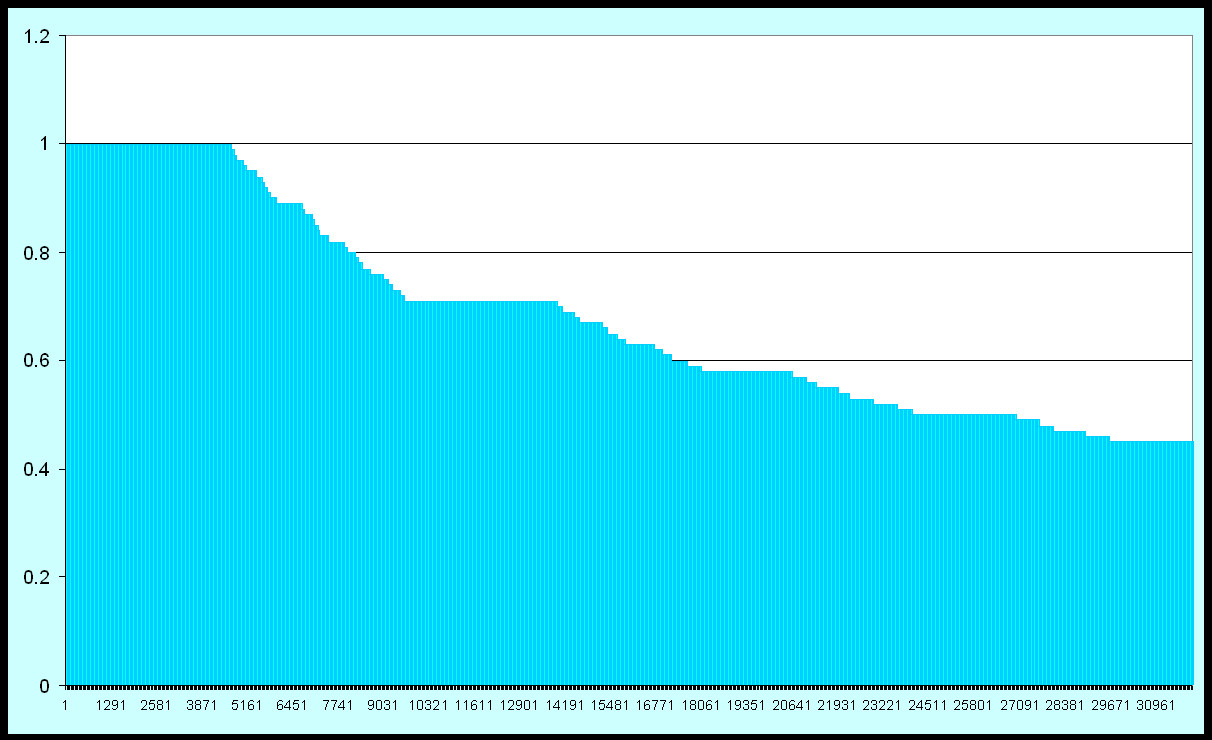
       Again, the vertical axis is the cosine similarity between the term vectors with a value of one indicating complete similarity and a value of zero indicating no similarity between the vectors. The difference in the graphs of the frequency based term-term correlations and the Cosine based similarity calculation is due to the larger number of significantly co-occurring low frequency terms which produce a higher cosine value. These co-occurrences, due to the lower underlying frequencies of the constituent terms, ranked much lower in a frequency only calculation. The several plateau's in the graph are due to the rounding of the output to only 2 digits to the right of the decimal point.

       Alternatively, we can use the the Jaccard similarity (see above) formula which normalizes with respect to the number of occurrences. The Jaccard values range between 0 and 1. With this approach, if some term k occurs six times in the collection and some term h occurs five times and they co-occur zero times, the result is zero. If, however, they co-occur five times (the maximum), and they each occur once in each per document, the result is 5/(6+5-5) or 0.833. Similarly, if they each occur six times, once per document and have a co-occurrence of six times, the result is 6/(6+6-6) or 1.000. As can be seen, this formula, like the cosine formula, takes into account the number of times each term occurs independently of the number of co-occurrences.

       The Wikipedia results are here and the OSU Medline results are here.

    2. Modified Basic Indexing - Position Specific

       Another modification to improve term-term detection would involve retaining during document scanning the relative positions of the words with respect to one another in the collection. Then, when calculating the term-term matrix, proximity can be taken into account. If you add a new matrix to the scanning code above in addition to '^doc()' named ^p(DocNbr,Word,Position) which in the third index position, retains for each word in each document the position(s) which the word occurs in relative to the beginning of the document (abstracts and titles), it becomes possible to attenuate the strength of co-occurrences by the proximity of the co-occurrence.

       Subsequently, the term-term calculation becomes: for each document k, for each term i in k, for each other term j where j is alphabetically higher than i, for each position m each position m of term i, and each position n of term j, calculate and sum weights for ^tt(i,j) based on the distance between the terms. The distance is calculated with the formula:

       set dd=$zlog(1/$zabs(m-n)*20+1)\1

       which yields values of:

       $zabs(m-n)=1 result=3
       $zabs(m-n)=2 result=2
       $zabs(m-n)=3 result=2
       $zabs(m-n)=4 result=1
       $zabs(m-n)=5 result=1
       $zabs(m-n)=6 result=1
       $zabs(m-n)=7 result=1
       $zabs(m-n)=8 result=1
       $zabs(m-n)=9 result=1
       $zabs(m-n)=10 result=1
       $zabs(m-n)=11 result=1
       $zabs(m-n)=12 result=0
       $zabs((m-n)=13 result=0
       $zabs(m-n)=14 result=0
       $zabs(m-n)=15 result=0

       Thus, words immediately next to one another receive a score of three while words more than eleven positions apart receive a score of zero. For each pair {i,j} a third level index is summed which is the signed difference between m and n. Eventually, a positive or negative value for this term indicates a preference for which term appears first most often. Values of zero or near zero indicate that the terms appear in no specific order relative to one another. The program then calculates a histogram giving the number of term pairs at increasing scores (see link below). For example, there were nearly 400,000 word combinations the sum of whose scores was one. Alternatively, there was one pair of words whose co-occurrence score sum, calculated as above, was 1,732 (coron and artery). The length of the histogram bars are based on the logarithm of the value displayed to the left so as to make the graph more readable.

       Proximity Weighted Term-Term Correlation Matrix

       #!/usr/bin/mumps #+++++++++++++++++++++++++++++++++++++++++++++++++++++++++++++++++++ #+ #+ Mumps Information Storage and Retrieval Software Library #+ Copyright (C) 2005 by Kevin C. O'Kane #+ #+ Kevin C. O'Kane #+ okane@cs.uni.edu #+ #+ #+ This program is free software; you can redistribute it and/or modify #+ it under the terms of the GNU General Public License as published by #+ the Free Software Foundation; either version 2 of the License, or #+ (at your option) any later version. #+ #+ This program is distributed in the hope that it will be useful, #+ but WITHOUT ANY WARRANTY; without even the implied warranty of #+ MERCHANTABILITY or FITNESS FOR A PARTICULAR PURPOSE. See the #+ GNU General Public License for more details. #+ #+ You should have received a copy of the GNU General Public License #+ along with this program; if not, write to the Free Software #+ Foundation, Inc., 59 Temple Place, Suite 330, Boston, MA 02111-1307 USA #+ #++++++++++++++++++++++++++++++++++++++++++++++++++++++++++++++++++++++ # proximity.mps March 13, 2008 set %=$zStopInit("good") // loads stop list into a C++ container open 1:"translated.txt,old" if '$test write "translated not found",! halt use 1 set p=0 set doc=0 set M=20000 for do . if doc>M set doc=doc-1 break . use 1 . set word=$zzScan . if '$test break . if word="xxxxx115xxxxx" set off=$zzScan,doc=$zzScan,p=0 quit // new abstract . if '$zStopLookup(word) quit // is "word" in the good list . set p=p+1 . set ^p(doc,word,p)="" use 5 close 1 set ^DocCount(1)=doc # ttx term-term correlation matrix # calculate term-term proximity coefficients within env words kill ^tt //* delete any old term-term correlation matrix write !!,"Term-Term Correlation [ttx.mps] ",$zd,! #++++++++++++++++++++++++++++++++++++++++++++++++++++++++++++++++++++++ # for each document k, sum the co-occurrences of words i and j #++++++++++++++++++++++++++++++++++++++++++++++++++++++++++++++++++++++ set Wgt=0 set Wgtx=0 Open 1:"ttx.tmp,new" # for each document k set k="" for do . set k=$order(^p(k)) . if k="" break # for each term i in p k . set i="" . for do .. set i=$order(^p(k,i)) .. if i="" break # for each other term j in doc k .. set j=i .. for do ... set j=$order(^p(k,j)) ... if j="" break # for each position m of term i in doc k ... set m="" ... for do .... set m=$order(^p(k,i,m)) .... if m="" break # for each position n of term j in doc k .... set n="" .... for do ..... set n=$order(^p(k,j,n)) ..... if n="" break # calculate and store weight based on proximity ..... set dd=$zlog(1/$zabs(m-n)*20+1)\1 ..... if dd<1 quit ..... if '$Data(^tt(i,j)) set ^tt(i,j)=dd,^tt(i,j,1)=n-m,Wgtx=Wgtx+1,Wgt=Wgt+dd ..... else set ^tt(i,j)=^tt(i,j)+dd,^tt(i,j,1)=^tt(i,j,1)+(n-m),Wgt=Wgt+dd do graph # normalize set max=0 set i="" for do . set i=$order(^tt(i)) . if i="" break . set j=i . for do .. set j=$order(^tt(i,j)) .. if j="" break .. if ^tt(i,j)>max set max=^tt(i,j) # set max=WgtFactor/100*dm\1 set max=max*.1\1 # build other diagonal matrix set i="" for do . set i=$order(^tt(i)) . if i="" break . set j=i . for do .. set j=$order(^tt(i,j)) .. if j="" break .. if ^tt(i,j)<max kill ^tt(i,j) .. else set ^tt(j,i)=^tt(i,j) set i="" set Wgt=Wgt/Wgtx write !,"Average term-term correlation: ",Wgt,! # write "Maximum term-term correlation: ",dm,! # write "Weight factor percentage: ",WgtFactor,! write "Discard term-term connections with weight less than: ",max,! for do . set i=$order(^tt(i)) . if i="" break . if $order(^tt(i,""))="" quit . write !!,"*** ",i,!," " . set j="" . for do .. set j=$order(^tt(i,j)) .. if j="" break .. if i=j quit .. else do ... write:$x>65 !," " ... write " ",j,"[",^tt(i,j),"]" ... if j]i do .... Use 1 .... write $Justify(^tt(i,j),6),?10,i," ",j,?50,^tt(i,j,1),! .... Use 5 write !! Close 1 set i=$zsystem("sort -n -r <ttx.tmp > ttx.rank") //* shell command set i=$zsystem("rm ttx.tmp") //* shell command write "Dump data: ",$zcd("ttx.dmp"),! write $zd,! halt graph write !,"Graphs",! kill ^hx kill ^hxx kill ^hr set i="" set k=0 for do . set i=$order(^tt(i)) . if i="" break . set j="" . for do .. set j=$order(^tt(i,j)) .. if j="" break .. set k=k+1 .. set ^hr(k)=^tt(i,j) set i=0 set dm=0 for do . set i=$order(^hr(i)) . if i="" break . if ^hr(i)>dm set dm=^hr(i) for j=1:1:dm set ^hx(j)=0 set i=0 for do . set i=$order(^hr(i)) . if i="" break . set j=^hr(i) . set ^hx(j)=^hx(j)+1 set hxmax=0 set j=$order(^hx("")) for i=j:1:dm set ^hxx(i)=^hx(i) set ^hx(i)=$zlog(^hx(i)+1) if ^hx(i)>hxmax set hxmax=^hx(i) write !,"Logarithmic Histogram Showing Number of Term Pairs for levels of Correlation Strength",!! write " Corr Words",!! set j=$order(^hx("")) for i=j:1:dm do . set k=^hx(i)/hxmax*100\1 . if ^hx(i)>0 do .. set k=k+1 .. write $Justify(i,5),$j(^hxx(i),7)," " .. for m=1:1:k write "*" .. write ! quit

       Full results are prox.gz and http://www.cs.uni.edu/~okane/source/ISR/medline.ttx.ranked The first column is the sum of the proximity scores followed by the words followed by the summation of the ordering factor. A negative number indicates the words most often occur in reverse order to that shown.

       As can be seen, a proximity based Term-Term matrix yields substantially better results although it is considerably more expensive to calculate in terms of time and space. The example was calculated on the first 10,000 documents in the data base.

    3. Term-Term clustering

       Terms can be grouped into clusters using the results of the term-term matrix above. In a single link clustering system, a term is added to a cluster if it is related to one term already in the cluster.

       #!/usr/bin/mumps #++++++++++++++++++++++++++++++++++++++++++++++++++++++++++++++++++++++ #+ #+ Mumps Bioinformatics Software Library #+ Copyright (C) 2004, 2005, 2006, 2008 by Kevin C. O'Kane #+ #+ Kevin C. O'Kane #+ anamfianna@earthlink.net #+ okane@cs.uni.edu #+ #+ #+ This program is free software; you can redistribute it and/or modify #+ it under the terms of the GNU General Public License as published by #+ the Free Software Foundation; either version 2 of the License, or #+ (at your option) any later version. #+ #+ This program is distributed in the hope that it will be useful, #+ but WITHOUT ANY WARRANTY; without even the implied warranty of #+ MERCHANTABILITY or FITNESS FOR A PARTICULAR PURPOSE. See the #+ GNU General Public License for more details. #+ #+ You should have received a copy of the GNU General Public License #+ along with this program; if not, write to the Free Software #+ Foundation, Inc., 59 Temple Place, Suite 330, Boston, MA 02111-1307 USA #+ #++++++++++++++++++++++++++++++++++++++++++++++++++++++++++++++++++++++ # clustertt.mps March 8, 2009 kill ^clstr kill ^x open 1:"tmp,new" use 1 for w1="":$order(^tt(w1)):"" do . for w2=w1:$order(^tt(w1,w2)):"" do .. write ^tt(w1,w2)," ",w1," ",w2,! close 1 set %=$zsystem("sort -n -r < tmp > tmp.sorted") open 1:"tmp.sorted,old" set c=1 for do . use 1 . read a // correlation word1 word2 . if '$test break . set score=$p(a," ",1) . set w1=$p(a," ",2) . set w2=$p(a," ",3) . if w1=w2 quit . set f=1 # ^x() is a two dimensional array that contains, at the second level, # a list of clusters to which the word (w1) belongs # ^cluster() is the cluster matrix. Each row (s) is a cluster # numbered 1,2,3 ... The second level is a list of the words # in the cluster. # The following # code runs thru all the clusters first for w1 (w1) and # adds w2 to those clusters w1 belongs to. It # repeats the process for w2. If a word pair are not # assigned to some cluster (f=1), they are assigned to a new # cluster and the cluster number is incremented (c) . if $d(^x(w1)) for s="":$order(^x(w1,s)):"" do .. set ^clstr(s,w2)="" .. set ^x(w2,s)="" .. set f=0 . if $d(^x(w2)) for s="":$order(^x(w2,s)):"" do .. set ^clstr(s,w1)="" .. set ^x(w1,s)="" .. set f=0 . if f do .. set ^clstr(c,w1)="" set ^x(w1,c)="" .. set ^clstr(c,w2)="" set ^x(w2,c)="" .. set c=c+1 # print the clusters close 1 use 5 write "number of clusters: ",c,!! for cx="":$order(^clstr(cx)):"" do . write cx," cluster",! . for w1="":$order(^clstr(cx,w1)):"" do .. use 5 write w1," " . write !!

       The results for a 20,000 abstract run are http://www.cs.uni.edu/~okane/source/ISR/medline.cluster-tt

    4. Construction of Term Phrases (Salton83, pages 84-89)

       Salton notes that recall can be improved if additional, related terms are added to a query. Thus, a query for 'antenna' will result in more hits in the data base if the related term 'aerial' is added. An increase in recall, however, is often accompanied by a decrease in precision. So, while 'aerial' is a commonly used synonym for 'antenna', as in 'television aerial', it can also refer to a dance move, a martial arts move, skiing, various musical groups and performances, and any activity that is done at a height (e.g., aerial photography). Thus, adding it to a query with antenna has the potential to introduce many extraneous hits.

       Identification of phrases, however, has the potential to increase precision. These are composite terms of high specificity - such as 'television aerial' noted above. While both 'television' and 'aerial' individually are broad terms, the phrase 'television aerial' or 'television antenna' is quite specific. When a phrase is identified, it becomes a single term in the document vector.

       Phrases can be identified by both syntactic and statistical methods. While techniques that take into account term proximity as well as co-occurrence such as suggested above, Salton suggests the following simpler formula for construction of term phrases:

       ^Cohesion(i,j) = SIZE_FACTOR * (^tt(i,j)/(^dict(i)*^dict(j)))

       The code to perform the cohesion calculation is here

       #!/usr/bin/mumps #+++++++++++++++++++++++++++++++++++++++++++++++++++++++++++++++++++ #+ #+ Mumps ISR Software Library #+ Copyright (C) 2006, 2008 by Kevin C. O'Kane #+ #+ Kevin C. O'Kane #+ anamfianna@earthlink.net #+ okane@cs.uni.edu #+ #+ #+ This program is free software; you can redistribute it and/or modify #+ it under the terms of the GNU General Public License as published by #+ the Free Software Foundation; either version 2 of the License, or #+ (at your option) any later version. #+ #+ This program is distributed in the hope that it will be useful, #+ but WITHOUT ANY WARRANTY; without even the implied warranty of #+ MERCHANTABILITY or FITNESS FOR A PARTICULAR PURPOSE. See the #+ GNU General Public License for more details. #+ #+ You should have received a copy of the GNU General Public License #+ along with this program; if not, write to the Free Software #+ Foundation, Inc., 59 Temple Place, Suite 330, Boston, MA 02111-1307 USA #+ #++++++++++++++++++++++++++++++++++++++++++++++++++++++++++++++++++++++ # cohesion.mps March 25, 2010 # phrase construction open 1:"tmp,new" use 1 for i=$order(^tt(i)) do . set j=i . for do .. set j=$o(^tt(i,j)) .. if j="" break .. set c=^tt(i,j)/(^dict(i)*^dict(j))*100000\1 .. if c>0 write c," ",i," ",j,! shell sort -nr < tmp > cohesion.results shell rm tmp

       The OSU Medline results are here: http://www.cs.uni.edu/~okane/source/ISR/medline.cohesion.sorted.gz and the Wikipedia results are here: http://www.cs.uni.edu/~okane/source/ISR/wiki.cohesion.sorted.gz .

       Salton notes that this procedure can sometimes result in unwanted connections such as 'Venetian blind' and 'blind Venetian'. For that reason, the aggregate relative order of the terms, as shown above, can help to decide when two terms are seriously linked. That is, if the order is strongly in favor of on term preceding another, this indicates a probable phrase; on the other hand, if the relative order is in neither direction, this is probably not a phrase.

24. Document-Document Matrices

    It is also possible to construct Document-Document Matrices giving the correlation between all documents which have significant similarities with one another. Such a matrix can be used to generate document clusters and for purposes of document browsing by permitting the user to navigate related documents to the one being viewed. That is, if a user finds on of the retrieved articles of particular interest, a Document-Document matrix can be used to quickly identify other documents related to the document of interest. The source code is shown below and the Wikipedia results are http://www.cs.uni.edu/~okane/source/ISR/wiki.dd2.gz and the OSU Medline results are http://www.cs.uni.edu/~okane/source/ISR/medline.dd2.gz.

    The program only calculates the cosines between documents that share at least one term rather than between all possible documents.

    #!/usr/bin/mumps #+++++++++++++++++++++++++++++++++++++++++++++++++++++++++++++++++++ #+ #+ Mumps ISR Software Library #+ Copyright (C) 2007, 2008 2010 by Kevin C. O'Kane #+ #+ Kevin C. O'Kane #+ anamfianna@earthlink.net #+ okane@cs.uni.edu #+ #+ #+ This program is free software; you can redistribute it and/or modify #+ it under the terms of the GNU General Public License as published by #+ the Free Software Foundation; either version 2 of the License, or #+ (at your option) any later version. #+ #+ This program is distributed in the hope that it will be useful, #+ but WITHOUT ANY WARRANTY; without even the implied warranty of #+ MERCHANTABILITY or FITNESS FOR A PARTICULAR PURPOSE. See the #+ GNU General Public License for more details. #+ #+ You should have received a copy of the GNU General Public License #+ along with this program; if not, write to the Free Software #+ Foundation, Inc., 59 Temple Place, Suite 330, Boston, MA 02111-1307 USA #+ #++++++++++++++++++++++++++++++++++++++++++++++++++++++++++++++++++++++ #!/usr/bin/mumps # docdoc5.mps March 27, 2010 write !!,"Document-document matrix ",$zd,! if '$data(%1) set min=2 else set min=%1 if '$data(%2) set wgt=0.8 else set wgt=%1 kill ^dd for w=$order(^idf(w)) do . if ^idf(w)<min quit . for d1=$order(^index(w,d1)) do .. set d2=d1 .. for do ... set d2=$order(^index(w,d2)) ... if d2="" break ... if $data(^dd(d1,d2)) quit ... set ^dd(d1,d2)=$zzCosine(^doc(d1),^doc(d2)) for d1=$order(^dd(d1)) do . for d2=$order(^dd(d1,d2)) do .. if ^dd(d1,d2)<wgt kill ^dd(d1,d2) .. else set ^dd(d2,d1)=^dd(d1,d2) for d1=$order(^dd(d1)) do . write !,d1,": ",?10 . set k=0 . for d2=$order(^dd(d1,d2)) do .. write d2,"(",$justify(^dd(d1,d2),1,2),") " .. set k=k+1 .. if k#7=0 write !,?10

25. File and Document Clustering (Salton83, pages 215-222)

    (see also: advanced clustering)

    1. Hierarchical Clustering
    2. Web Document Clustering: A Feasibility Demonstration (pdf)
    3. Document Clustering
    4. Hierarchical Document Clustering (pdf)
    5. A comparative study of generative methods for document clustering (pdf)
    6. Demonstration of hierarchical document clustering (pdf)
    7. Relationship-based Clustering and Cluster Ensembles for High-dimensional Data Mining, Alexander Strehl

    The program cluster.mps uses a single link clustering technique similar to that used in the term clustering above. The program generates and then reads a file of document-document correlations sorted in reverse (highest to lowest) correlation order.

    #!/usr/bin/mumps #++++++++++++++++++++++++++++++++++++++++++++++++++++++++++++++++++++++ #+ #+ Mumps Bioinformatics Software Library #+ Copyright (C) 2004, 2005, 2006, 2008 by Kevin C. O'Kane #+ #+ Kevin C. O'Kane #+ anamfianna@earthlink.net #+ okane@cs.uni.edu #+ #+ #+ This program is free software; you can redistribute it and/or modify #+ it under the terms of the GNU General Public License as published by #+ the Free Software Foundation; either version 2 of the License, or #+ (at your option) any later version. #+ #+ This program is distributed in the hope that it will be useful, #+ but WITHOUT ANY WARRANTY; without even the implied warranty of #+ MERCHANTABILITY or FITNESS FOR A PARTICULAR PURPOSE. See the #+ GNU General Public License for more details. #+ #+ You should have received a copy of the GNU General Public License #+ along with this program; if not, write to the Free Software #+ Foundation, Inc., 59 Temple Place, Suite 330, Boston, MA 02111-1307 USA #+ #++++++++++++++++++++++++++++++++++++++++++++++++++++++++++++++++++++++ # cluster.mps March 9, 2008 kill ^clstr kill ^x open 1:"tmp,new" use 1 for d1="":$order(^dd(d1)):"" do . for d2=d1:$order(^dd(d1,d2)):"" do .. write ^dd(d1,d2)," ",d1," ",d2,! close 1 set %=$zsystem("sort -n -r < tmp > tmp.sorted") open 1:"tmp.sorted,old" set c=1 for do . use 1 . read a // correlation doc1 doc2 . if '$test break . set score=$p(a," ",1) . set seq1=$p(a," ",2) . set seq2=$p(a," ",3) . if seq1=seq2 quit . set f=1 # ^x() is a two dimensional array that contains, at the second level, # a list of clusters to which the document number (seq1) belongs # ^cluster() is the cluster matrix. Each row (s) is a cluster # numbered 1,2,3 ... The second level is a list of the document # numbers of those documents in the cluster. The following # code runs thru all the clusters first for doc1 (seq1) and # adds seq2 (doc2) to those clusters doc1 belongs to. It # repeats the process for seq2 (doc2). If a doc pair are not # assigned to some cluster (f=1), they are assigned to a new # cluster and the cluster number is incremented (c) . if $d(^x(seq1)) for s="":$order(^x(seq1,s)):"" do .. set ^clstr(s,seq2)="" .. set ^x(seq2,s)="" .. set f=0 . if $d(^x(seq2)) for s="":$order(^x(seq2,s)):"" do .. set ^clstr(s,seq1)="" .. set ^x(seq1,s)="" .. set f=0 . if f do .. set ^clstr(c,seq1)="" set ^x(seq1,c)="" .. set ^clstr(c,seq2)="" set ^x(seq2,c)="" .. set c=c+1 # print the clusters close 1 open 1:"osu.medline,old" if '$test write "missing translated.txt",! halt use 5 write "number of clusters: ",c,!! for cx="":$order(^clstr(cx)):"" do . use 5 write cx," cluster",! . for seq1="":$order(^clstr(cx,seq1)):"" do .. use 1 set %=$zseek(^doc(seq1)) read title .. use 5 write $e(title,1,120),! . use 5 write !

    The results for OSU Medline are here: http://www.cs.uni.edu/~okane/source/ISR/medline.clusters.gz and the Wikipedia results are here: http://www.cs.uni.edu/~okane/source/ISR/wiki.clusters.gz.

26. Web Page Access - Building a Simple Keyword Based Logical Expression Server Page

    The following will outline the process to build an interactive web page to access the data. At this point, we assume that the data base has been processed and the appropriate global array vectors and matrices exist. The following program will access the data base:

    #!/usr/bin/mumps #++++++++++++++++++++++++++++++++++++++++++++++++++++++++++++++++++++++ #+ #+ Mumps ISR Software Library #+ Copyright (C) 2000, 2005, 2006 by Kevin C. O'Kane #+ #+ Kevin C. O'Kane #+ anamfianna@earthlink.net #+ okane@cs.uni.edu #+ #+ #+ This program is free software; you can redistribute it and/or modify #+ it under the terms of the GNU General Public License as published by #+ the Free Software Foundation; either version 2 of the License, or #+ (at your option) any later version. #+ #+ This program is distributed in the hope that it will be useful, #+ but WITHOUT ANY WARRANTY; without even the implied warranty of #+ MERCHANTABILITY or FITNESS FOR A PARTICULAR PURPOSE. See the #+ GNU General Public License for more details. #+ #+ You should have received a copy of the GNU General Public License #+ along with this program; if not, write to the Free Software #+ Foundation, Inc., 59 Temple Place, Suite 330, Boston, MA 02111-1307 USA #+ #++++++++++++++++++++++++++++++++++++++++++++++++++++++++++++++++++++++ # webFinder.mps March 23, 2008 html Content-type: text/html &!&! set t=$zd1 html <html><body bgcolor=silver> if '$data(query) set query="" html <center><img src=http://sidhe.cs.uni.edu/moogle.gif border=0><br> html <form name="f1" method="get" action="webFinder.cgi"> html <input type="text" name="query" size=50 maxlength=128 value="&~query~"> html &nbsp <input type="submit" value="Search"> html </form> html <form name="f1" method="get" action="webFinder.cgi"> html <input type="hidden" name="query" value="###"> html &nbsp <input type="submit" value="I'm Feeling Sick"> html </form></center> write ! if query="" write "</body></html>",! halt if query="###" do . set w="" . for i=1:1 do .. set w=$order(^dict(w)) .. if w="" break . set j=$r(i-1) . set w="" . for i=1:1:j do .. set w=$order(^dict(w)) . set query=w kill ^d kill ^query do $zwi(query) set wx=0 for w=$zwp do . if w?.P continue . set ^query(w)=1 . for d="":$order(^index(w,d)):"" set ^d(d)="" Set i=$zwi(query) set exp="" for w=$zwp do . if w="" break . if $find("&()",w) set exp=exp_w continue . if w="|" set exp=exp_"!" continue . if w="~" set exp=exp_"'" continue . set exp=exp_"$d(^doc(d,"""_w_"""))" write "<br>",exp,"<br>",! kill ^dx set max=0 set count=0 for d="":$order(^d(d)):"" do . set $noerr=1 // corrected for interpreter use Apr 22, 2009 . set %=@exp . if $noerr<0 write "Query parse error.</body></html>",! halt . if %>0 do .. set C=$zzCosine(^query,^doc(d)) .. set ^dx(C,d)="" .. set count=count+1 write count," pages found - top 10 shown<hr><tt><pre>",! set d="" set i=0 open 1:"translated.txt,old" if '$test write "translated.txt not found",! halt for do . if i>10 break . set d=$order(^dx(d),-1) . if d="" break . for dd="":$order(^dx(d,dd)):"" do .. set i=i+1 .. if i>10 break .. write $j(d,6,3)," " .. write "<a href=display.cgi?ref=",dd,">" .. use 1 do $zseek(^doc(dd)) read title use 5 .. write $j(dd,6)," ",$extract(title,1,90),"</a>",! write "<pre><p>Time used: ",$zd1-t,"<br>",! html </body></html> kill ^d kill ^dx halt

    In the program, the interpreter decodes the incoming environment variable QUERY_STRING set by the web server. It instantiates variable names with values as found in "xxx=yyy" figures contained in QUERY_STRING. In particular, this application receives a variable named "query" which is either empty, the value "###" or an optionally parenthesized logical expression involving keywords.

    In the case where "query" is missing or empty, only the form text box is returned to the browser. In the case where the value of "query" is "###", a random word is selected from the vocabulary and this work becomes the value of "query"

    The value of "query" is processed first to extract all the words provided. A global array vector named "query" is constructed with the words as indices. For each word, all the document numbers associated with the word in ^index() are fetched and stored in a temporary vector ^d(). When processing of all words is complete, the vector ^query() contains the words and the vector ^d() contains the document numbers of all documents that have one or more words in common with the query.

    Next, the query is rescanned and a Mumps string is built. For each word in the query, a entry of the form:

    $d(^doc(d,"word"))

    is constructed where the value of the word is enclosed in quotes. These are connected to other similar expressions by not (~), and (&), or (!), and parentheses. Note: the input vertical bar character (|) is converted to the Mumps exclamation point "or" character (!). For example, query:

    (ducks & chickens) | (rabbits & foxes)

    becomes:

    ($d(^doc(d,"ducks"))&$d(^doc(d,"chickens")))!($d(^doc(d,"rabbits"))&$d(^doc(d,"foxes")))

    Note: parsing of Mumps expressions is always left to right (no precedence) unless parentheses are used.

    Once the query has been re-written, the program cycles through each document number in ^d(). For each document number "d", the expression built from the query is executed interpretively and the result, zero or greater than zero, determines if the document should be processed further. If the result is greater than zero, the Cosine of the document vector and the query is calculated and stored in the temporary vector ^dx(cosine,docNbr). This two part index is used so that the same Cosine value can have multiple document numbers linked to it.

    Finally, the document titles (^t()) are printed in reverse cosine order. Each title is expressed as a link to the program display.cgi which will ultimately display the abstract.

    The program produces output such as (OSU Medline example):

    

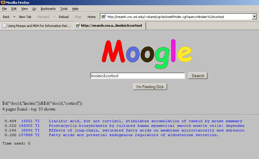
    A live (or dead - depends on the server) version can be seen by clicking here .

    Unfortunately, the program above depends upon the user to be familiar with the vocabulary used in the data base. A user who spells a word incorrectly or uses a similar but different synonym is out of luck. However, there are several ways to improve data base navigation. The program above can be extended with a front end that permits point-and-click browsing for terms and term combinations. In order to do this, we used the results of the term-term matrix above with a lower threshold (thereby increasing the number of possible word combinations). The term-term matrix was used as input to a program that produced an alphabetic two level hierarchical organization of the terms that became input for a point-and-click web based display procedure.

    #!/usr/bin/mumps #++++++++++++++++++++++++++++++++++++++++++++++++++++++++++++++++++++++ #+ #+ Mumps ISR Software Library #+ Copyright (C) 2000, 2005, 2008 by Kevin C. O'Kane #+ #+ Kevin C. O'Kane #+ anamfianna@earthlink.net #+ okane@cs.uni.edu #+ #+ #+ This program is free software; you can redistribute it and/or modify #+ it under the terms of the GNU General Public License as published by #+ the Free Software Foundation; either version 2 of the License, or #+ (at your option) any later version. #+ #+ This program is distributed in the hope that it will be useful, #+ but WITHOUT ANY WARRANTY; without even the implied warranty of #+ MERCHANTABILITY or FITNESS FOR A PARTICULAR PURPOSE. See the #+ GNU General Public License for more details. #+ #+ You should have received a copy of the GNU General Public License #+ along with this program; if not, write to the Free Software #+ Foundation, Inc., 59 Temple Place, Suite 330, Boston, MA 02111-1307 USA #+ #++++++++++++++++++++++++++++++++++++++++++++++++++++++++++++++++++++++ # ttfolder.mps January 2, 2008 for i=0:1:25 do . set a=$c(97+i) . set w1=$order(^dfi(a)) . if $e(w1,1,1)'=a continue . write a,! . write """blank.html"" target=right",!! . for w1=a:$order(^dfi(w1)):"" do .. if $e(w1,1,1)'=a break .. if ^dfi(w1)<3 quit .. write ". ",w1,! .. write ". ""blank.html"" target=right",!! .. write ".. ",w1,! .. write ".. ""webFinder.cgi?query=",$zh(w1),""" ",!! .. if '$data(^tt(w1)) quit .. for w2="":$order(^tt(w1,w2)):"" do ... write ".. ",w1," & ",w2,! ... write ".. ""webFinder.cgi?query=",$zh(w1_"&"_w2),""" ",!!

    First, we use a program (above) that extracts term pairs from the term-term matrix. The OSU Medline results are here http://www.cs.uni.edu/~okane/source/ISR/medline.ttfolder.gz.

    The output from the above is input to a program that produces dynamic, web based folders. Each entry is two lines with a blank line following. The first line is the text to be displayed and the second line is the action or page to be performed if the text is clicked. The number of dots preceding each line determines the level in the hierarchy of the entry. The file is organized at the highest level by letters of the alphabet (a through z) and the n by words beginning with that letter. Beneath each word is a list of words with a significant correlation to the higher term, as determined by the term-term matrix.

    The program that reads the output of the above and builds the hierarchy is here:

    #!/usr/bin/mumps # ++++++++++++++++++++++++++++++++++++++++++++++++++++++++++++++++++ # # Information Storage and Retrieval Indexer # Copyright (C) 2000, 2005, 2006, 2008 by Kevin C. O'Kane # # Kevin C. O'Kane # anamfianna@earthlink.net # okane@cs.uni.edu # # # This program is free software; you can redistribute it and/or modify # it under the terms of the GNU General Public License as published by # the Free Software Foundation; either version 2 of the License, or # (at your option) any later version. # # This program is distributed in the hope that it will be useful, # but WITHOUT ANY WARRANTY; without even the implied warranty of # MERCHANTABILITY or FITNESS FOR A PARTICULAR PURPOSE. See the # GNU General Public License for more details. # # You should have received a copy of the GNU General Public License # along with this program; if not, write to the Free Software # Foundation, Inc., 59 Temple Place, Suite 330, Boston, MA 02111-1307 USA # # ++++++++++++++++++++++++++++++++++++++++++++++++++++++++++++++++++++++ # tab.mps January 2, 2008 set lev(0)="0000\Browser Tree" set ord=1000 for Do . read cmd . if '$Test break . if cmd="" continue . for i=0:1:10 if $extract(cmd,i+1,i+1)'="." quit . for do .. if $extract(cmd,1,1)="."!($extract(cmd,1,1)=" ") set cmd=$extract(cmd,2,512) quit .. break . set lev(i)=cmd . read order // line2 . for do .. if $extract(order,1,1)="."!($extract(order,1,1)=" ") set order=$extract(order,2,512) quit .. break . set x="" . for j=0:1:i-1 set x=x_""""_lev(j)_"""," . set x=x_""""_lev(i)_"""" . set x="^lib("_x . set %=x_")" . set order="@"_order . set @%=order . write %," -> ",order,! halt

    The results for OSU Medline are here: http://www.cs.uni.edu/~okane/source/ISR/medline.tab.gz.

    Finally, once the internal hierarchy is built, the program that displays the indices is here:

    #!/usr/bin/mumps #++++++++++++++++++++++++++++++++++++++++++++++++++++++++++++++++++++++ #+ #+ Mumps Web Software Library #+ Copyright (C) 2000, 2005, 2006, 2008 by Kevin C. O'Kane #+ #+ Kevin C. O'Kane #+ anamfianna@earthlink.net #+ okane@cs.uni.edu #+ #+ #+ This program is free software; you can redistribute it and/or modify #+ it under the terms of the GNU General Public License as published by #+ the Free Software Foundation; either version 2 of the License, or #+ (at your option) any later version. #+ #+ This program is distributed in the hope that it will be useful, #+ but WITHOUT ANY WARRANTY; without even the implied warranty of #+ MERCHANTABILITY or FITNESS FOR A PARTICULAR PURPOSE. See the #+ GNU General Public License for more details. #+ #+ You should have received a copy of the GNU General Public License #+ along with this program; if not, write to the Free Software #+ Foundation, Inc., 59 Temple Place, Suite 330, Boston, MA 02111-1307 USA #+ #++++++++++++++++++++++++++++++++++++++++++++++++++++++++++++++++++++++ # index.mps January 2, 2008 znumber html Content-type: text/html &!&!<html> html <head><title>Mumps Web Folders</title></head> html <body vlink=darkblue link=darkblue bgcolor=silver>&! html <!-- Mumps Web Folders, Copyright (C) 2001 Kevin C. O'Kane &! html Mumps Web Folders comes with ABSOLUTELY NO WARRANTY; &! html This is free software, and you are welcome to redistribute it&! html under certain conditions as set forth in the GNU GPL -->&! if '$data(^count(1)) set ^count(1)=1 set ^date(1)=$zd set date=$zd else set ^count(1)=^count(1)+1 set date=^date(1) if '$data(ml) set ml=1 set line=0 if '$data(array) set array="lib" set %1="<a href=""index.cgi?array="_array_"&ml=" set %2="<a href=" set cls="<img align=top src=""/folder03.gif"" border=0>" set lev=1,bx=0,ep=0,c(0)="" for i=0:1:20 do . set b(i)="" . set x="a"_i . set a(i)="" . if $data(@x) set b(i)=@x,ep=i do layer html <center> html </body></html> halt layer set x(lev)="^"_array_"(" set AFLG=0 for i=1:1:lev do . set x(lev)=x(lev)_"a("_i_")" . if i'=lev set x(lev)=x(lev)_"," set x(lev)=x(lev)_")" set a(lev)=-1 if b(lev)'="",lev<ml do . set a(lev)="" a1 set a(lev)=$order(@x(lev)) if a(lev)="" set lev=lev-1 quit set p="array="_array if lev>bx do parm1 set n="<br>",nn="" for i=1:1:lev-1 set n=n_"..." for i=1:1:lev-1 set nn=nn_"..." if $data(@x(lev))>1,ml>lev,b(lev)=a(lev) do . html </a><br><a name=node&~lev~></a> . write nn," ",%1,lev set line=0 . do parm . Html "> . Html <img align=middle src="/folder05.gif" border=0> . set line=line+1 . set AFLG=1 . goto a3a if $data(@x(lev))=1,lev=ml do . write n . set n="" . goto a3a if $data(@x(lev))'=1 do . if line>25 do .. write "<br>" set line=0 .. write nn,%1,lev+1 . else write n,%1,lev+1 . do parm . write """>",cls set line=line+1 . set AFLG=1 a3a if AFLG do tok if 'AFLG do . if $extract(@x(lev),1,1)="@" do .. set p=$extract(@x(lev),2,100) . write %2,p . html > . if $data(@x(lev))=1 set line=line+1 html &~n~&nbsp;<img src=/blueball.gif border=0 align=top>&nbsp; . do tok . Html </a> if lev<ml do . if $data(@x(lev))>1,b(lev)=a(lev) do .. if $extract(@x(lev),1,1)="@" do ... set p=$extract(@x(lev),2,100) .. write %2,p set line=line+1 .. Html > .. Html </a>&! if @x(lev)="" goto a2a set x=@x(lev) if lev<ml goto a2a ; print only low level if $extract(x,1,1)="@" do . set x=$extract(x,2,255) a2a if lev>bx do parm1 if $data(@x(lev))>1,ml>lev,b(lev)=a(lev) do . set lev=lev+1 . do layer . goto a1 goto a1 parm for i=1:1:lev quit:a(i)=-1 write "&a",i,"=",$zh(a(i)) html #node&~lev~ quit # tok write !,$piece(a(lev)," ",2,99) tok write !,a(lev) if AFLG html </a> quit parm1 set bx=lev for i=1:1:lev set c(i)=a(i) quit

    Which produces an initial browser display such as the following:

    

    Upon clicking on the letter "o", the display becomes:

    

    Upon clicking on the "obstructive" link, the display becomes:

    

    Upon clicking the button "obstructive & apnea" the webFinder program is invoked with the keys selected (and'ed) and the display becomes:

    

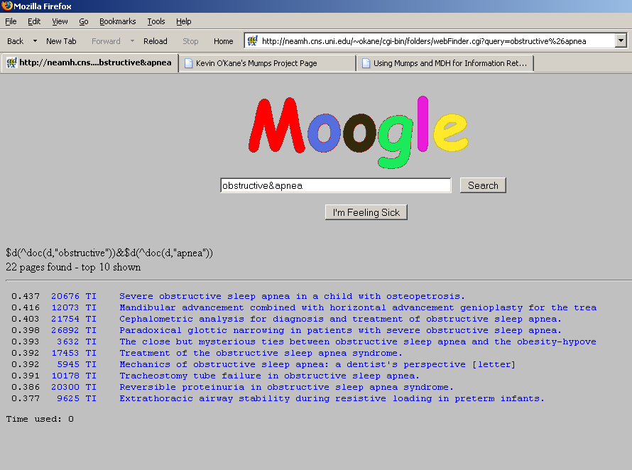
    If the user clicks the first retrieved title, the program display.mps is run:

    #!/usr/bin/mumps #+++++++++++++++++++++++++++++++++++++++++++++++++++++++++++++++++++ #+ #+ Mumps ISR Software Library #+ Copyright (C) 2005, 2006, 2008 by Kevin C. O'Kane #+ #+ Kevin C. O'Kane #+ okane@cs.uni.edu #+ #+ #+ This program is free software; you can redistribute it and/or modify #+ it under the terms of the GNU General Public License as published by #+ the Free Software Foundation; either version 2 of the License, or #+ (at your option) any later version. #+ #+ This program is distributed in the hope that it will be useful, #+ but WITHOUT ANY WARRANTY; without even the implied warranty of #+ MERCHANTABILITY or FITNESS FOR A PARTICULAR PURPOSE. See the #+ GNU General Public License for more details. #+ #+ You should have received a copy of the GNU General Public License #+ along with this program; if not, write to the Free Software #+ Foundation, Inc., 59 Temple Place, Suite 330, Boston, MA 02111-1307 USA #+ #++++++++++++++++++++++++++++++++++++++++++++++++++++++++++++++++++++++ # display.mps March 23, 2008 html Content-type: text/html &!&! html <html><body bgcolor=silver> if '$data(ref) write "Missing reference number </body></html>" halt open 1:"osu.medline,old" if '$test write "osu.medline not found",! halt use 1 set %=$zseek(^doc(ref)) html <table bgcolor=lightsteelblue align=center width=60% border><tr><td><i>Mesh Headings:</i><br> set flg=0 for do . use 1 . read a // find the title . if a="" do .. html No abstract available .. html </table></body></html> .. halt . if $extract(a,1,3)="MH " do .. use 5 .. set i=$find(a,"/") .. if i=0 set i=255 .. else set i=i-2 .. set a=$extract(a,7,i) .. do $zwi(a) .. for ww=$zwp do ... if ww?.p continue ... set wx=ww ... if $data(^lib($e(wx,1,1),wx)) do .... html <a href=index.cgi? .... html array=lib&ml=3&a1=&~$e(wx,1,1)~&a2=&~wx~#node2> .... write ww,"</a> " ... else write ww," " . if $extract(a,1,3)="TI " do .. use 5 .. do $zwi($extract(a,7,255)) .. html <tr><td><i>Title:&nbsp;</i> .. for ww=$zwp do ... set wx=ww ... if $data(^lib($e(wx,1,1),wx)) do .... html <a href=index.cgi? .... html array=lib&ml=3&a1=&~$e(wx,1,1)~&a2=&~wx~#node2> .... write ww,"</a> " ... else write ww," " .. html </td><tr><td><i>Abstract:</i>&nbsp; . if $extract(a,1,3)="AB " for do .. use 5 .. do $zwi($extract(a,7,255)) .. for ww=$zwp do ... set wx=ww ... if $data(^lib($e(wx,1,1),wx)) do .... html <a href=index.cgi? .... html array=lib&ml=3&a1=&~$e(wx,1,1)~&a2=&~wx~#node2> .... write ww,"</a> " ... else write ww," " .. use 1 read a .. if a=""!($extract(a,1,3)'=" ") set flg=1 break . if flg break use 5 html <tr><td><i>Related Documents</i>: set d="" for do . set d=$order(^dd(ref,d)) . if d="" break . use 1 set %=$zseek(^doc(d)) . for do .. use 1 .. read a // find the title .. if a="" do ... html </table></body></html> ... halt .. if $extract(a,1,3)="TI " do ... use 5 ... html <br><a href=display.cgi?ref= ... write d,">",d,"</a> " ... do $zwi($extract(a,7,255)) ... for ww=$zwp do .... set wx=ww .... if $data(^lib($e(wx,1,1),wx)) do ..... html <a href=index.cgi? ..... html array=lib&ml=3&a1=&~$e(wx,1,1)~&a2=&~wx~#node2> ..... write ww,"</a> " .... else write ww," " html </table></body></html>

    The program above accesses the original source text from the OSU Medline data base. In an earlier step, the program sourceOffsets.mps was run to extract the offsets of the original text.

    and the display becomes:

    

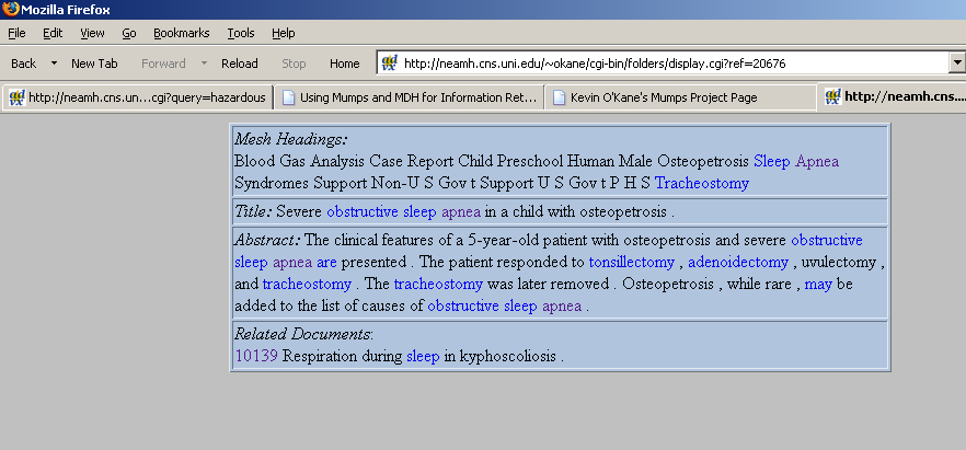
    The web index program is capable of multiple levels of hierarchy but the combinatorics of word combinations become very large unless care is taken only to display very common, broadly appearing terms at the higher levels.

    In the above display, if the user clicks on a a highlighted word, they are taken to the initial display of folders with the folder for the keyword clicked open. Also listed at the bottom are the article numbers of related documents (from the doc-doc matrix). Clicking on one of the document numbers will display the selected document with its keywords highlighted.

    An online demo of the above programs is available here (depending on server availability). Note: this operates on a student server and may be down or operate very slowly at times.

    Indexing Text Features in Genomic Repositories

    Since the widespread adoption of the Internet in the early 1990's, there has been explosive growth in machine readable data bases both in the form of online data bases as well as web page based content. Readily accessible indexable content now easily ranges into terabytes. When indexing very large data sets, special procedures should be used to maximize efficiency. The following is a case study based on indexing the text content of genomic data bases.

    Since 1990, the massive growth in genetic and protein databases has created a pressing need for tools to manage, retrieve and analyze the information contained in these libraries. Traditional tools to organize, classify and extract information have often proved inadequate when confronted with the overwhelming size and density of information which includes not only sequence and structural data, but also text that describes the data's origin, location, species, tissue sample, journal articles, and so forth. As of this writing, the NCBI (National Center for Biotechnology Information, part of the National Institutes of Health) GenBank library alone consists of nearly 84 billion bytes of data and it is only one of several data banks storing similar information. The scope and size of these databases continues to rapidly grow and will continue to do so for many years to come as will the demand for access.

    A typical entry in GenBank looks like: (from: ftp://ftp.ncbi.nih.gov/genbank/ )

    Web Abstract Display Program

    LOCUS AAB2MCG2 1276 bp DNA linear PRI 23-AUG-2002 DEFINITION Aotus azarai beta-2-microglobulin precursor exons 2, 3, and complete cds. ACCESSION AF032093 AF032094 VERSION AF032093.1 GI:3287308 KEYWORDS . SEGMENT 2 of 2 SOURCE Aotus azarai (Azara's night monkey) ORGANISM Aotus azarai Eukaryota; Metazoa; Chordata; Craniata; Vertebrata; Euteleostomi; Mammalia; Eutheria; Primates; Platyrrhini; Cebidae; Aotinae; Aotus. REFERENCE 1 (bases 1 to 1276) AUTHORS Canavez,F.C., Ladasky,J.J., Muniz,J.A., Seuanez,H.N., Parham,P. and Cavanez,C. TITLE beta2-Microglobulin in neotropical primates (Platyrrhini) JOURNAL Immunogenetics 48 (2), 133-140 (1998) MEDLINE 98298008 PUBMED 9634477 REFERENCE 2 (bases 1 to 1276) AUTHORS Canavez,F.C., Ladasky,J.J., Seuanez,H.N. and Parham,P. TITLE Direct Submission JOURNAL Submitted (31-OCT-1997) Structural Biology, Stanford University, Fairchild Building Campus West Dr. Room D-100, Stanford, CA 94305-5126, USA COMMENT On or before Jul 2, 1998 this sequence version replaced gi:3265029, gi:3265028. FEATURES Location/Qualifiers source 1..1276 /organism="Aotus azarai" /mol_type="genomic DNA" /db_xref="taxon:30591" mRNA join(AF032092.1:<134..200,66..344,1023..>1050) /product="beta-2-microglobulin precursor" CDS join(AF032092.1:134..200,66..344,1023..1036) /codon_start=1 /product="beta-2-microglobulin precursor" /protein_id="AAC52107.1" /db_xref="GI:3289965" /translation="MARFVVVALLVLLSLSGLEAIQRXPKIQVYSRHPAENGKPNFLN CYVSGFHPSDIEVDLLKNGKKIEKVEHSDLSFSKDWSFYLLYYTEFTPNEKDEYACRV SHVTLSTPKTVKWDRNM" mat_peptide join(AF032092.1:194..200,66..344,1023..1033) /product="beta-2-microglobulin" intron <1..65 /number=1 variation 3 /note="allele 1" /replace="g" exon 66..344 /number=2 intron 345..1022 /number=2 exon 1023..1050 /number=3 intron 1051..>1276 /number=3 ORIGIN 1 caagttatcc gtaattgaaa taccctggta attaatattc atttgtcttt tcctgatttt 61 ttcaggtrct ccaaagattc aggtttactc acgtcatccg gcagagaatg gaaagccaaa 121 ttttctgaat tgctatgtgt ctgggtttca tccgtccgac attgaagttg acttactgaa 181 gaatggaaag aaaattgaaa aagtggagca ttcagacttg tctttcagca aggactggtc 241 tttctatctc ttgtactaca ccgagtttac ccccaatgaa aaagatgagt atgcctgccg 301 tgtgagccat gtgactttat caacacccaa gacagtaaag tggggtaagt cttacgttct 361 tttgtaggct gctgaaagtt gtgtatgggt agtcatgtca taaagctgct ttgatataaa 421 aaaaattcgt ctatggccat actgccctga atgagtccca tcccgtctga taaaaaaaaa 481 tcttcatatt gggattgtca gggaatgtgc ttaaagatca gattagagac aacggctgag 541 agagcgctgc acagcattct tctgaaccag cagtttccct gcagctgagc agggagcagc 601 agcagcagtt gcacaaatac atatgcactc ctaacacttc ttacctactg acttcctcag 661 ctttcgtggc agctttaggt atatttagca ctaatgaaca tcaggaaggt ataggccttt 721 ctttgtaaat ccttctatcc tagcatccta taatcctgga ctcctccagt actctctggc 781 tggattggta tctgaggcta gtaggtgggg cttgttcctg ctgggtagct ccaaacaagg 841 tattcatgga taggaacagc agcctatttt gccagcctta tttcttaata gttttagaaa 901 tctgttagta cgtggtgttt tttgttttgt tttgttttaa cacagtgtaa acaaaaagta 961 catgtatttt aaaagtaaaa cttaatgtct tcctttttct ttctccactg tctttttcat 1021 agatcgaaac atgtaaccag catcatggag gtaagttctt gaccttaatt aaatgttttt 1081 tgtttcactg gggactattt atagacagcc ctaacatgat aaccctcact atgtggagaa 1141 cattgacaga gtagcatttt agcaggcaaa gaggaatcct atagggttac attccctttt 1201 cctgtggagt ggcatgaaaa aggtatgtgg ccccagctgt ggccacatta ctgactctac 1261 agggagggca aaggaa

    An annotated example GenBank record is available here while a complete description of the NCBI data base can be found here.

    Currently, retrieval of genomic data is mainly based on well-established programs such as FASTA (Pearson, 2000, see: ) and BLAST (Altschul, 1997), that match candidate nucleotide sequences against massive libraries of sequence acquisitions. There have been few efforts to provide access to genomic data keyed to the extensive text annotations commonly found in these data sets. Among the few systems that deal with keyword based searching are the proprietary SRS system (Thure and Argos, 1993a, 1993b) and PIR (Protein Information Resource) (Wu 2003). These are limited, controlled vocabulary systems whose keys are from manually prepared annotations. To date, there have been no systems reported to directly generate indices from the genomic data sets themselves. The reasons for this are several: the very large size of the underlying data sets, the size of intermediate indexing files, the complexity of the data, and the time required to perform the indexing.

    The system described here, MARBL (Mumps Analysis and Retrieval from Bioinformatics Libraries), is an application to integrate multiple, very large, genomic, databases into a unified data repository through open-source components; and to provide fast, web-based keyword based access to the contents.

    Sequences retrieved by MARBL can be post-processed by FASTA (Pearson, 2000), Smith-Waterman (Smith, 1981) and elements of EMBOSS (the European Molecular Biology Open Software Suite). While FASTA and, especially, Smith-Waterman, are more sensitive (Shpaer et al. 1996) than BLAST, they are also more time consuming. However, by first extracting from the larger database a subset of candidate accessions, the number of sequences to be aligned by these algorithms can be reduced significantly with corresponding reduction in the overall processing time.

    Implementation

    Most genomic databases include, in addition to nucleotide and protein sequences, a wealth of text information in the form of descriptions, keywords, annotations, hyper-links to text articles, journals and so forth. In many cases, the text attachments to the data are greater in size that the actual sequence data. Identifying the important keyword terms from this data and assigning a relative weight to these terms is one of the problems addressed in this system.

    While indexing can be approached from the perspective of assignment to pre-existing categories and hierarchies such as the National Library of Medicine MeSH (Medical Subject Headings) (Hazel, 1997), derivative indexing is better able to adapt to changes in a rapidly evolving discipline as the terms are dynamically extracted directly from the source material rather than waiting for manual analysis. Existing keyword based genomic retrieval systems are primarily based on assignment indexing whereas the approach taken here is based on derivative indexing, where both queries and documents are encoded into a common intermediate representation and metrics are developed to calculate the coefficients of similarity between queries and documents. Documents are ranked according to their computed similarity to the query and presented to the user in rank order. Several systems employing this and related models have been implemented such as Smart (Salton, 1968, 1971, 1983, 1988), Instruct (Wade, 1988), Cansearch (Pollitt, 1987) and Plexus (Vickery, 1987a, 1987b). More recently, these approaches have been used to index Internet web pages and provide collaborative filtered recommendations regarding similar texts to book buyers at Amazon.com (Linden, 2003).

    In this system, genomic accessions are represented by vectors that reflect accession content through descriptors derived from the source text by analysis of word usage (Salton,1968, 1971, 1983, 1988; Willett, 1985; Crouch, 1988). This approach can be further enhanced by identifying clusters of similar documents (El-Hamdouchi et al.,1988, 1989). Similarly, term-term co-occurrence matrices can be constructed to identify similar or related terms and these can be automatically included into queries to enhance recall or to identify term clusters. Other techniques based on terms and queries have also been explored (Salton, 1988; Williams, 1983).

    The vector model is rooted in the construction of document vectors consisting of the weights of each term in each document. Taken collectively, the document vectors constitute a document-term matrix whose rows are document vectors. A document-term matrix can have millions of rows, more than 22 million in GenBank case, and thousands of columns (terms), more than 500,000 in GenBank. This yields a matrix with potentially trillions of possible elements which must be quickly addressable not by numeric indices but by text keys. Additionally, to enhance information retrieval speed, an inverted matrix of the same size is needed which doubles the overall storage requirements. Fortunately, however, both matrices are very sparse.

    Given the nature of the problem, namely, manipulating massive, character string indexed sparse matrices, we implemented the system in Mumps.

    Using Mumps global arrays, an accession-term matrix appears in the Mumps language as an array of the form: ^D(Accession,Term) where both Accession and Term are text strings. The matrix is indexed row-wise by accession codes and column-wise by text derived terms. This approach vastly simplifies implementation of the basic information storage and retrieval model. For example, the main Mumps indexing program used in the basic protocol described below is about 76 lines of code (excluding in-line C functions). The highly concise nature of the Mumps language permits rapid deployment and minimizes maintenance problems that would be the case with more complex coding systems.

    FASTA (Pearson, 2000) and Smith-Waterman (Smith and Waterman, 1981) are sequence alignment procedures to match candidate protein or NA sequences to entries in a database. Sequences retrieved as a result of text searches with the system described here can be post-processed by FASTA and the Smith-Waterman. Of these, the Smith-Waterman algorithm is especially sensitive and accurate but also relatively time consuming. Using this system to isolate candidate sequences by text keywords and subsequently processing the resulting subset of the larger database, results in considerable time savings. In our experiments we used the Smith-Waterman program available as part of the FASTA package developed by W. R. Pearson (Pearson 2000). Additionally, the output of this system is compatible with the many genomic analysis programs found in the open source EMBOSS collection.

    The system software is compatible with several genomic database input formats, subject to preprocessing by filters. In the example presented here, the NCBI GenBank collection was used. GenBank consists of accessions which contain sequence and related data collected by researchers throughout the world.

    Two protocols were developed to index the GenBank data sets. Initially, we tried a direct, single step, vector space model protocol that constructed the accession-term matrix directly from the GenBank files. However, experiments revealed that this approach was unacceptably slow when used with large data sets. This resulted in the development of a multi-step protocol that performed the same basic functions but as a series of steps designed to improve overall processing speed. The discussion below centers on the multi-step protocol although timing results are given for both models. The work was performed on a Linux based, dual processor hyper-threaded Pentium Xeon 2.20 GHz system with 1 GB of main memory and dual 120 GB EIDE 7,200 rpm disk drives.

    The entire GenBank data collection consisted of approximately 83.5 GB of data at the time of these experiments. When working with data sets of smaller size, relatively straightforward approaches to text processing can be used with confidence. However, when working with data sets of very large dimensions, it soon became apparent that special strategies would be needed in order to reduce the complexity of the processing problem. During indexing, as the B-tree grew, delays due to I/O became significant when the size of the data set exceeded the amount of physical memory available. At that point, the memory I/O cache became inadequate to service I/O requests without significant actual movement of data to and from external media. When this happened, CPU utilization was observed to drop to very low values while input/output activity grew to system maximum. Once page thrashing began, overall progress to index the data set slowed dramatically.

    In order to avoid this problem, the multi-step protocol was devised in which the indexing tasks were divided into multiple steps and sort routines were employed in order to prepare intermediate data files so that at each stage where the database was being loaded into the B-tree, the keys were presented to the system in ascending key order thus inducing an effectively sequential data set build and eliminating page thrashing. While this process produced a significant number of large intermediate files, it was substantially faster than unordered key insertion.

    Data Sets

    The main data sets used were from the NCBI GenBank collection (ftp://ftp.ncbi.nlm.nih.gov):

    1. The GenBank short directory, gbsdr.txt consisting of locus codes which, at this writing, is approximately 1.45 billion bytes in length and has approximately 18.2 million entries.
    2. The nucleotide data, the accessions, are stored in over 300 gzip compressed files. Each file is about 220 megabytes long and consists of nucleotide accessions. We pre-process each file with a filter program that extracts text and other information. Pre-processing results in a format similar to the EMBL (European Micro Biology Laboratory) format and this makes for faster processing in subsequent steps as well as greatly reducing disk storage requirements. For example, the file gbbct1.seq, currently 250,009,587 bytes in length, reduced to 8,368,295 bytes after pre-processing.
    3. Optionally, a list of NCBI manually derived multi-word keys from the file gbkey.idx (502,549,211 bytes). Processing of these keys is similar to that of derived keys but only a default, minimum weight is produced.
    4. In addition to text found in the accessions, GenBank, as well as many other data resources, contains links to on-line libraries of journal articles, books, abstract and so forth. These links provided additional sources of text keys related to the accessions in the originating database.

    Multiple Step Protocol

    The multiple step protocol, shown in Figure 1, separated the work into several steps and was based on the observation that using system sort facilities to preprocess data files resulted in much faster database creation since the keys can be loaded into the B-tree database in ascending key order. This observation was founded in an early experiment in which an accession-term matrix was constructed by loading the keys from a 5 million accessions file sorted by ascending accession key. The load procedure itself used a total of 1,032 seconds (17.2 minutes). On the other hand, loading the keys directly from a file not sorted by accession was 7.1 times slower requiring 7,333 seconds (122.2 minutes) to load.

    
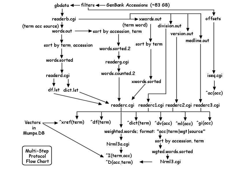
    Figure 1

    The main text analysis procedure reads the filtered version of the accession files. Lines of text were scanned, punctuation and extraneous characters were removed, words matching entries in the stop list were discarded, and, finally, words were processed to remove suffixes and consolidated into groups based on word stems (readerb.cgi). Each term was written to an output file (words.out) along with its accession code and a code indicating the source of the data. A second file was also produced that associated each processed stem along with the original form of the term (xwords.out). The output files were sorted concurrently. The xwords.out file was sorted by term with duplicate entries discarded while the words.out file was sorted to two output files: words.sorted, ordered by term then accession code, and words.sorted.2 ordered by accession code then term.

    The file words.sorted was processed to count word usage (readerd.cgi). As the file was ordered by term then accession code, multiple occurrences of a word in a document appear on successive lines. The program deleted words whose overall frequency of occurrence was too low or high. Files df.lst and dict.lst were produced which contain, respectively, for each term, the number of accessions in which it appears in, and the total number of occurrences.

    The file words.sorted.2 (sorted by accession code and term) was processed by readerg.cgi to produce words.counted.2 which generated for each accession, the number of times each term occurred in an accession and a string of code letters giving the original sources of the term (from the original input line codes). This file was ordered by accession and term.

    The files xwords.sorted, df.lst, dict.lst and words.counted.2 were processed by readerc.cgi to produce internal data vectors and an output file named weighted.words which contained the accession code, term, the calculated inverse document frequency weight of the term, and source code(s) for the term. If the calculated weight of a term in an accession was below a threshold, it was discarded. Since the input file words.counted.2 was ordered by accession then by term, the output file weighted.words was also ordered by accession then term.

    Finally, the Nrml3a.cgi constructed the term-accession matrix (^I) from the term sorted file weighted.words and Nrml3.cgi built the accession-term matrix (^D) from wgted.words.sorted which was ordered by accession and term. In this final step, the database assumed its full size and it was this step that is most critical in terms of time. As each of the matrices were ordered according to their first, then second indices, the B-tree was built in ascending key order.

    Retrieval

    Retrieval is via a web page interface or an interactive keyboard based program. Queries are expressed as logical expressions of terms, possibly including wildcards. Queries may be restricted to data particular sources (title, locus, etc.) or specific divisions (ROD, PRI, etc). When a query is submitted to the system it is first expanded to include related terms for any wildcards. The expression is converted into a Mumps expression and candidate accession codes of those accessions containing terms from the query are identified. The Mumps expression is applied to each identified candidate accession. A similarity coefficient between the accession and the query is calculated based on the weight of the terms in the accessions using a simple similarity formula.

    From the accessions retrieved, the user can view the original NCBI accession page, save the accession list for further reference or convert the accessions to FASTA format and match the accessions against a candidate sequence with the FASTA or the Smith-Waterman algorithm. By means of the GI code from the VERSION field in the original GenBank accession, a user can access full data concerning the retrieved accession directly from NCBI. Also stored is the Medline access code which provides direct entry into the Medline database for the accession.

    Retrieval times are proportional to the amount of material retrieved, the complexity of the query, and the number of accessions in which each query term appears.. For specific queries that retrieve only a few accessions, processing times less than 1 second are typical.

    Results and Discussion

    Some overall processing statistics for the two protocols are given in Table 1. As can be seen, the multi-step protocol performed significantly better than the basic protocol.

    Table 1 - Processing Time Statistics (in minutes)
    Accessions Processed	1,000,000	5,000,000	22,318,882
    Multi-Step Protocol	63.9	350.8	2,016.1
    Basic Protocol	246.9	1,735.61	6994.7

    The dimensions of the final matrices are potentially of vast size: 22.3 million by 501,614 in this case. Potentially, this implies a matrix of 11.5 trillion elements. However, the matrix is very sparse and the file system stores only those elements which actually exist. After processing the entire GenBank, the actual database was only 23 GB although at its largest, before compaction of unused space, it reached 44 GB.

    Evaluation of information retrieval effectiveness from a data set of this size is clearly difficult as there are few benchmarks against which to compare the results. However, NCBI distributes a file of keyword phrases with GenBank gbkey.idx (502,549,211 bytes). This file contains submission author assigned keyword phrases and associated accession identifiers. Of the 48,023 unique keys in gbkey.idx (after removal of special characters and words less than three characters in length), 26,814 keys were the same as the keys selected by MARBL. The 21,209 keys that differed were, for the most part, words of very high or low frequency that the system rejected due to preset thresholds. Alternatively, the MARBL system identified and retained a highly specific 501,614 terms, many of which were specific codes used to identify genes.

    When comparing the accessions linked to keywords in gbkey.idx with MARBL derived accessions, it was clear that MARBL discovered vastly more linkages than the NCBI file identified. For example, the keyword zyxin (the last entry in gbkey.idx) was linked to 4 accessions by gbkey.idx but MARBL detected 336 accessions. In twelve other queries based on terms randomly selected from gbkey.idx, MARBL found more accessions than were listed in gbkey.idx in nine cases and the same number in three cases. On average, each MARBL derived keyword points to 130.34 accessions whereas gbkey.idx keys, on average, points to 6.80 accessions.

    We compared MARBL with BLAST by entering the nucleotide sequence of a Bacillus anthracis bacteriophage that was of interest to a local researcher. BLAST retrieved 24 accessions, with one scoring 1,356, versus the next highest with a score of 50. The highest scoring accession was the correct answer, while the remainder were noise. When we entered the phrase anthracis & bacteriophage to the MARBL information retrieval package, only one accession was retrieved, the same one that received the highest score from BLAST. BLAST took 29 seconds, MARBL information retrieval took 10 seconds. It should be noted, however, that BLAST searches are not based on keywords but on genomic sequences.

    Mumps is an excellent text indexing implementation language (O'Kane, 1992). Mumps programs are concise and are easily maintained and modified. The string indexed global arrays, underpinned by the effectively unlimited file sizes supported by the BDB, make it possible to design very large, efficient systems with minimal effort. In all, there were 10 main indexing routines with a total of 930 lines of Mumps code (including comments) for an average of 93 lines of code per module. On the other hand, the C programs generated by the Mumps compiler amounted to 21,146 lines of code, not counting many thousands of lines in run-time support and database routines. The size of the C routines is comparable to reported code sizes for other information storage and retrieval projects such as Wade (1988) who reports that Instruct as approximately 6,000 lines of Pascal code, and Plexus (Vickery and Brooks, 1987a) reported as approximately 10,000 lines although, due to differences in features, these figures should not be used for direct comparisons.

    An example of this system in its current state can be seen here.

27. N-gram encoding (Salton83, pages 93-94) During World War II, n-grams, fixed length consecutive series of "n" characters, were developed by cryptographers to break substitution ciphers. Applying n-grams to indexing, the text, stripped of non-alphabetic characters, is treated as a continuous stream of data that is segmented into non-overlapping fixed length words. These words can then form the basis of the indexing vocabulary.

    In the following experiment, the OSU TREC9 data base, is read and the text reduced to non-overlapping 3 letter n-grams. First, the input text is pre-processed to remove non-alpha characters and converted to lower case. The result is written in a FASTA format consisting of a title line beginning with a ">" followed by the title of the article followed by a long single line of text comprising the text and body of the article converted as noted above. (Note: if the lines of text exceed 2,500 characters, the Mumps Compiler configure parameter --with-strmax=val parameter will need to be increased from its default value of 2500.)

    Conversion of TREC9 Data Base to FASTA Format

    #+++++++++++++++++++++++++++++++++++++++++++++++++++++++++++++++++++ #+ #+ Mumps ISR Software Library #+ Copyright (C) 2007 by Kevin C. O'Kane #+ #+ Kevin C. O'Kane #+ okane@cs.uni.edu #+ #+ #+ This program is free software; you can redistribute it and/or modify #+ it under the terms of the GNU General Public License as published by #+ the Free Software Foundation; either version 2 of the License, or #+ (at your option) any later version. #+ #+ This program is distributed in the hope that it will be useful, #+ but WITHOUT ANY WARRANTY; without even the implied warranty of #+ MERCHANTABILITY or FITNESS FOR A PARTICULAR PURPOSE. See the #+ GNU General Public License for more details. #+ #+ You should have received a copy of the GNU General Public License #+ along with this program; if not, write to the Free Software #+ Foundation, Inc., 59 Temple Place, Suite 330, Boston, MA 02111-1307 USA #+ #++++++++++++++++++++++++++++++++++++++++++++++++++++++++++++++++++++++ # fasta.mps April 1, 2007 open 1:"osu.medline,old" if '$test write "osu.medline file not found",! halt set f=0 for do . use 1 . read line . if '$test halt . if $e(line,1,2)="TI" use 5 write:f ! write "> ",$e(line,7,256),!,$$cvt(line) set f=1 quit . if $e(line,1,2)'="AB" quit . use 5 write $$cvt(line) . for do // for each line of the abstract .. use 1 read line .. if '$test use 5 write ! halt // no more input .. if line="" break .. use 5 write $$cvt(line) . use 5 write ! . set f=0 halt cvt(line) set buf="" for i=7:1:$l(line) do . if $e(line,i)?1A set buf=buf_$e(line,i) set buf=$zlower(buf) quit buf

    A substantially faster version, written in C:

    Conversion of TREC9 Data Base to FASTA Format

    // #+++++++++++++++++++++++++++++++++++++++++++++++++++++++++++++++++++ // #+ // #+ Mumps ISR Software Library // #+ Copyright (C) 2007 by Kevin C. O'Kane // #+ // #+ Kevin C. O'Kane // #+ okane@cs.uni.edu // #+ // #+ // #+ This program is free software; you can redistribute it and/or modify // #+ it under the terms of the GNU General Public License as published by // #+ the Free Software Foundation; either version 2 of the License, or // #+ (at your option) any later version. // #+ // #+ This program is distributed in the hope that it will be useful, // #+ but WITHOUT ANY WARRANTY; without even the implied warranty of // #+ MERCHANTABILITY or FITNESS FOR A PARTICULAR PURPOSE. See the // #+ GNU General Public License for more details. // #+ // #+ You should have received a copy of the GNU General Public License // #+ along with this program; if not, write to the Free Software // #+ Foundation, Inc., 59 Temple Place, Suite 330, Boston, MA 02111-1307 USA // #+ // #++++++++++++++++++++++++++++++++++++++++++++++++++++++++++++++++++++++ // // # MDH-fasta.cpp April 1, 2007 #include <stdio.h> #include <stdlib.h> #include <ctype.h> #include <assert.h> #include <string.h> void cvt(char *line, char *buf) { int i,j; buf[0] = '\0'; j = 0; for (i=6; line[i] != '\0'; i++) if (isalpha(line[i])) buf[j++] = tolower(line[i]); buf[j] = 0; } int main () { FILE *u1; char line[512],buf[8192]; int i,j,f; u1 = fopen("osu.medline","r"); assert (u1 != NULL); f=0; while (1) { if (fgets(line, 512, u1) == NULL) break; if (strncmp(line,"TI",2) == 0) { if (f) printf("\n"); printf("> %s",&line[6]); cvt (line, buf); printf("%s",buf); f=1; continue; } if (strncmp(line,"AB",2) != 0) continue; cvt(line,buf); printf("%s",buf); while (1) { if (fgets(line, 512, u1) == NULL) break; if (strlen(line) == 1) break; cvt(line,buf); printf("%s",buf); } printf("\n"); f=0; } return EXIT_SUCCESS; }

    The results look like the following:

    TREC9 Data Base in FASTA Format Example

    > The binding of acetaldehyde to the active site of ribonuclease: alterations in catalytic activity and effects of phosphate. thebindingofacetaldehydetotheactivesiteofribonucleasealterationsincatalyticactivityandeffectsofphosphateribonucleaseawasreacte dwithccacetaldehydeandsodiumcyanoborohydrideinthepresenceorabsenceofmphosphateafterseveralhoursofincubationatdegreescphstablea cetaldehydernaseadductswereformedandtheextentoftheirformationwassimilarregardlessofthepresenceofphosphatealthoughthetotalamoun tofcovalentbindingwascomparableintheabsenceorpresenceofphosphatethisactivesiteligandpreventedtheinhibitionofenzymaticactivitys eeninitsabsencethisprotectiveactionofphosphatediminishedwithprogressiveethylationofrnaseindicatingthatthereversibleassociation ofphosphatewiththeactivesitelysylresiduewasovercomebytheirreversibleprocessofreductiveethylationmodifiedrnasewasanalysedusingc protondecouplednmrspectroscopypeaksarisingfromthecovalentbindingofenrichedacetaldehydetofreeaminogroupsintheabsenceofphosphate wereasfollowsnhterminalalphaaminogroupppmbulkethylationatepsilonaminogroupsofnonessentiallysylresiduesppmandtheepsilonaminogro upoflysineattheactivesiteppminthespectrumofrnaseethylatedinthepresenceofphosphatethepeakatppmwasabsentwhenrnasewasselectivelyp remethylatedinthepresenceofphosphatetoblockallbuttheactivesitelysylresiduesandthenethylatedinitsabsencethesignalatppmwasgreatl ydiminishedandthatarisingfromtheactivesitelysylresidueatppmwasenhancedtheseresultsindicatethatphosphatespecificallyprotectedth eactivesitelysinefromreactionwithacetaldehydeandthatmodificationofthislysinebyacetaldehydeadductformationresultedininhibitiono fcatalyticactivity > Reductions in breath ethanol readings in normal male volunteers following mouth rinsing with water at differing temperatures reductionsinbreathethanolreadingsinnormalmalevolunteersfollowingmouthrinsingwithwateratdifferingtemperaturesbloodethanolconcen trationsweremeasuredsequentiallyoveraperiodofhoursusingalionaedalcolmeterinhealthymalesubjectsgivenoralethanolgkgbodywtreading sweretakenbeforeandafterrinsingthemouthwithwateratvaryingtemperaturesmouthrinsingresultedinareductioninthealcolmeterreadingsat allwatertemperaturestestedthemagnitudeofthereductionwasgreaterafterrinsingwithwateratlowertemperaturesthiseffectoccursbecauser insingcoolsthemouthanddilutesretainedsalivathisfindingshouldbetakenintoaccountwheneverbreathanalysisisusedtoestimatebloodethan olconcentrationsinexperimentalsituations > Does the blockade of opioid receptors influence the development of ethanol dependence? doestheblockadeofopioidreceptorsinfluencethedevelopmentofethanoldependencewehavetestedwhethertheopioidantagonistsnaloxonemgkgn altrexonemgkganddiprenorphinemgkgandtheagonistmorphinemgkggivensubcutaneouslyminbeforeethanolfordaysmodifytheethanolwithdrawal syndromeaudiogenicseizuresfollowingchronicethanolintoxicationinratswefoundthatnaloxonenaltrexoneanddiprenorphinemodifiedtheeth anolwithdrawalsyndromethesefindingsdonotruleoutthepossibilityofabiochemicallinkbetweentheactionofethanolandopiatesatthelevelof opioidreceptors

    Next, the text is read and and broken down into three character "words."

    Indexing using n-grams words

    #+++++++++++++++++++++++++++++++++++++++++++++++++++++++++++++++++++ #+ #+ Mumps Information Storage and Retrieval Software Library #+ Copyright (C) 2005, 2007 by Kevin C. O'Kane #+ #+ Kevin C. O'Kane #+ okane@cs.uni.edu #+ #+ #+ This program is free software; you can redistribute it and/or modify #+ it under the terms of the GNU General Public License as published by #+ the Free Software Foundation; either version 2 of the License, or #+ (at your option) any later version. #+ #+ This program is distributed in the hope that it will be useful, #+ but WITHOUT ANY WARRANTY; without even the implied warranty of #+ MERCHANTABILITY or FITNESS FOR A PARTICULAR PURPOSE. See the #+ GNU General Public License for more details. #+ #+ You should have received a copy of the GNU General Public License #+ along with this program; if not, write to the Free Software #+ Foundation, Inc., 59 Temple Place, Suite 330, Boston, MA 02111-1307 USA #+ #++++++++++++++++++++++++++++++++++++++++++++++++++++++++++++++++++++++ # shredder.mps March 28, 2007 open 1:"osu.fasta,old" set doc=1 for do . use 1 . read a . if '$t break . set ^t(doc)=a . read a . for do .. set word=$zShred(a,3) .. if word="" break .. set ^doc(doc,word)="" . set doc=doc+1 set %=$zzTranspose(^doc,^index)

    The following is a simple program to retrieve text based on 3 character n-grams. Note that the ShredQuery() function produces overlapping n-grams from the query.

    Program to Retrieve Text Based on 3 letter Encodings

    #+++++++++++++++++++++++++++++++++++++++++++++++++++++++++++++++++++ #+ #+ Mumps Information Storage and Retrieval Software Library #+ Copyright (C) 2005 by Kevin C. O'Kane #+ #+ Kevin C. O'Kane #+ okane@cs.uni.edu #+ #+ #+ This program is free software; you can redistribute it and/or modify #+ it under the terms of the GNU General Public License as published by #+ the Free Software Foundation; either version 2 of the License, or #+ (at your option) any later version. #+ #+ This program is distributed in the hope that it will be useful, #+ but WITHOUT ANY WARRANTY; without even the implied warranty of #+ MERCHANTABILITY or FITNESS FOR A PARTICULAR PURPOSE. See the #+ GNU General Public License for more details. #+ #+ You should have received a copy of the GNU General Public License #+ along with this program; if not, write to the Free Software #+ Foundation, Inc., 59 Temple Place, Suite 330, Boston, MA 02111-1307 USA #+ #++++++++++++++++++++++++++++++++++++++++++++++++++++++++++++++++++++++ # shredquery.mps 11/15/05 read "query: ",query for do . if $l(query)=0 break . set word=$$^ShredQuery(query,3) . if word="" break . set d="" . for do .. set d=$order(^index(word,d)) .. if d="" break .. if $data(^result(d)) set ^result(d)=^result(d)+1 .. else set ^result(d)=1 set d="" for do . set d=$order(^result(d)) . if d="" break . set ^ans($justify(^result(d),5),d)="" set sc="" set %=0 for do . set sc=$order(^ans(sc),-1) . if sc="" break . set d="" . for do .. set d=$order(^ans(sc,d)) .. if d="" break .. write sc," ",d," ",^title(d),! .. set %=%+1 .. if %>20 halt

    The above produces output of the form (longer titles truncated):

    Example Output

    sidhe:/r0/MEDLINE-TMP # shredquery.cgi query: alcohol 10 100214 > Lithium treatment of depressed and nondepressed alcoholics [see comments] 10 100502 > Alcohol effects on luteinizing hormone releasing hormone-stimulated anterior pituitary and gonadal hormones in women. 10 100656 > Is alcohol consumption related to breast cancer? Results from the Framingham Heart Study. 10 101146 > Hyaluronic acid and type III procollagen peptide in jejunal perfusion fluid as markers of connective tissue turnover. 10 101401 > Prevalence, detection, and treatment of alcoholism in hospitalized patients [see comments] 10 10210 > Alcoholic intemperance, coronary heart disease and mortality in middle-aged Swedish men. 10 102107 > Functional and structural changes in parotid glands of alcoholic cirrhotic patients. 10 103730 > Alcohol consumption and mortality in aging or aged Finnish men [published erratum appears in J Clin Epidemiol 1989;42(7):701] 10 103762 > The role of liquid diet formulation in the postnatal ethanol exposure of rats via mother's milk. 10 103913 > Comparative effectiveness and costs of inpatient and outpatient detoxification of patients with mild-to-moderate alcohol withdrawal ... 10 103926 > The effects of alcoholism on skeletal and cardiac muscle [see comments] 10 10407 > Genetic models of alcohol dependence. 10 10411 > Genetic control of liver alcohol dehydrogenase expression in inbred mice. 10 104287 > The generation of acetonemia/acetonuria following ingestion of a subtoxic dose of isopropyl alcohol. 10 10439 > Increased alcohol intake induced by chronic stimulants: is "orality" involved? 10 10440 > Naloxone attenuation of voluntary alcohol consumption. 10 10441 > Neonatal antidepressant administration suppresses concurrent active (REM) sleep and increases adult alcohol consumption in rats. 10 10444 > Is carbohydrate metabolism genetically related to alcohol drinking? 10 10449 > The antisocial and the nonantisocial male alcoholic--II. 10 10450 > Alcohol and ambience: social and environmental determinants of intake and mood. 10 10454 > Life events in the biography of French male and female alcoholics.

    The above example generates very large indexing files due to the large number of fragments extracted for each abstract. To be more effective, the distribution of the fragments using an algorithm such as the Inverse Document Frequency method should be used to rank fragments for their likely usefulness in resolving articles. In practice, as is the case when dealing with actual natural language text words, fragments whose distributions are very wide and very narrow can be deleted from the indexing set. (See the section below on application of IDF to genomic data.)

    Overview of Other Methods

28. Latent Semantic Model

    Essentially and term-term co-occurrence method used to augment queries. An execellent example of a very bad patent award (1988) - the underlying techniques have been around since the 1960's.

    References to Papers on LSI
    Wikipedia Entry on LSI

29. Single Term Based Indexing

    Reference: Salton 1983.

    Summary:

    • Single term methods view the collection as a set of individual terms.
    • Methodologies based on this approach seek to identify which terms are most indicative of content and to quantify the relative resolving power of each term.
    • Documents are generally viewed as vectors of terms weighted by the product of a term's frequency of occurrence in the document and its weight in the collection as a whole.
    • The vector space of a document collection may be treated as an hyperspace and the effect of a term on the space density may be taken as indicative of the term's resolving or discriminating power.
    • Documents may be clustered based on the similarities of their vector representations. Hierarchies of clusters may be generated.
    • Queries are treated as weighted vectors and the calculated similarity between a query vector and document vectors determines the ranking of a document in the results presented.
    • Answers to queries are ranked by recall and precision - measures of the degree of effectiveness of the methodology to find all documents in a collection relevant to a query and the degree to which irrelevant documents are included with relevant documents.
    • Queries may be enhanced by including terms whose usage patterns are similar to words in the original query.

30. Phrase Based Indexing
    • These are based on multiple words taken as phrases that are likely to convey greater context so as to improve precision.
    • Methods can involve thesauruses which group multiple words together into concept classes.
    • Methods can seek the identification of key phrases in a document. or construction of phrases from document context.

31. N-Gram Based Indexing

    N-grams

32. Example Code

    The following link is to a collection of Mumps code that performs the operations listed above: http://www.cs.uni.edu/~okane/source/ISR/ISR115Code.tgz .

33. Visualization

    An increasingly important aspect of IS&R is the ability to present the results to the user in a meaningful manner and interact with the user to refine his or her requests. In the early Salton experiments, queries and results were in text format only and generally entered, processed, and returned in batches. Since the widespread availability of the Internet as well and the general availability of graphical user interfaces, newer methods of rendering results can be explored. The following links give examples of several of these:

    1. Modern Information Retrieval Chapter 10: User Interfaces and Visualization - by Marti Hearst

    2. Visualizing the Non-Visual: spatial Analysis and Interaction with Information from Text Documents J.A. Wise, J.J. Thomas, K. Pennock, D. Lantrip, M. Pottier, A. Schur, and V. Crow (PDF file)

       Visualizing the Non-Visual: Spatial Analysis and Interaction with Information from Text Documents J.A. Wise, J.J. Thomas, K. Pennock, D. Lantrip, M. Pottier, A. Schur, and V. Crow (PowerPoint File)

    3. Internet browsing and searching: User evaluations of category map and Concept Space (PDF)

    4. Exploring the World Wide Web with Self-Organizing Map

    5. HIBROWSE interfaces

    6. Scatter/Gather clustering

34. Text Searching

35. Open Directory

    Open Directory Project

36. Text Searching in Genomic Data Bases
    1. Entrez/PubMed
    2. SRS

37. Applications to Genomic Data Bases

    In the past 15 years, genomics data bases have grown rapidly. These include both text and genetic information and the need to search them is central to research in areas such as genetic, drug discovery and medicine, to name a few.

    Genetic data bases include both natural language text as well as sequences of genetic information. Data bases containing genetic data bases are primarily divided into two types: those containing protein information and those containing DNA sequences. DNA sequence data bases usually consist of natural language text together with DNA sequence information over the nucleotide alphabet of bases {ACGT}. These letters stand for:

    1. Adenine
    2. Cytosine
    3. Guanine
    4. Thymine

    DNA itself is a double stranded helix with the nucleotides constituting the links across the strands (see: here)

    Protein sequence data bases are over the alphabet {ACDEFGHIKLMNPQRSTVWY} of amino acids. Sections of DNA are codes that are used to construct proteins. The order of the amino acids in a protein determine its shape, chemical activity and function.

    DNA substrings become proteins through a process of translation and transcription. The DNA is divided into three letter codons which select amino acids for incorporation into the protein being built.

    Over evolutionary time, DNA and resulting protein structures mutate. Thus, when searching either a protein or nucleotide data base, exact matches are not always the case. However, it has been observed that certain mutations are favored in nature while others are not. Generally speaking, this is because some mutations do not effect the functionality of the resulting proteins while other render the protein unusable.

    Many searching algorithms take evolutionary mutation into account through the use of substitution matrices. These give a score as to the probability of a given substitution of one amino acid for another based on observation in nature. The BLAST substitution matrices are typical. Different matrices are used to account for the amount of presumed evolutionary distance.

38. GenBank

    "GenBank is a component of a tri-partite, international collaboration of sequence databases in the U.S., Europe, and Japan. The collaborating database in Europe is the European Molecular Biology Laboratory (EMBL) at Hinxton Hall, UK, and in Japan, the DNA Database of Japan (DDBJ) in Mishima, Japan. Patent sequences are incorporated through arrangements with the U.S. Patent and Trademark Office, and via the collaborating international databases from other international patent offices. The database is converted to various output formats including the Flat File and Abstract Syntax Notation 1 (ASN.1) versions. The ASN.1 form of the data is included in www-Entrez and network-Entrez and is also available, as is the flat file, by anonymous FTP to 'ftp.ncbi.nih.gov'." (ftp://ftp.ncbi.nih.gov/genbank/README.genbank)

    1. Main GenBank FTP Site
    2. General Release Notes
    3. Feature Table Definitions
    4. Annotated Sample Record

39. EMBL/EBI (European Molecular Biology Laboratory/European Bioinformatics Institute

    "The European Bioinformatics Institute (EBI) is a non-profit academic organisation that forms part of the European Molecular Biology Laboratory (EMBL). The EBI is a centre for research and services in bioinformatics. The Institute manages databases of biological data including nucleic acid, protein sequences and macromolecular structures. The mission of the EBI is to ensure that the growing body of information from molecular biology and genome research is placed in the public domain and is accessible freely to all facets of the scientific community in ways that promote scientific progress." (from: http://www.ebi.ac.uk/Information/ )

    1. EBI Home Page
    2. EBI FTP Server

40. Alignment Algorithms

    In bioinformatics, a researcher identifies a protein or nucleotide sequence and wants to locate similar sequences in the data base. Some of the earliest methods used involve sequence alignment. Most direct sequence alignment techniques are very compute intensive and impractical to be applied with very large data bases. However, they represent the "gold standard" for sequence matching. The following is an historical overview of alignment algorithms and their evolution.

    • Elementary Sequence Alignment
      1. Dot Plots
      2. Needleman-Wunch Global Alignment
      3. Smith-Waterman Local Alignment
    • Outline of WN, Sellers, and SW algorithms
    • Needleman-Wunsch and Smith-Waterman
    • Smith-Waterman
    • Discussion of Blast, Fasta, and Smith-Waterman

41. Mumps Smith-Waterman Example

42. FASTA
    • FASTA Algorithm

43. BLAST (Basic Local Alignment Sequencing Tool)
    1. Blast HTML home page
    2. Blast FTP home page
    3. Blast Data Bases
    4. Substitution Matrices
    5. Blast Executables
    6. Blast Algorithm

44. Case Study: Indexing the "nt" Data Base

    This section explores the hypothesis that it is possible to identify genomic sequence fragments in large data bases whose indexing characteristics are comparable to that of a weighted vocabulary of natural language words. The Inverse Document Frequency (IDF) is a simple but widely used natural language word weighting factor that measures the relative importance of words in a collection based on word distribution. A high IDF weight usually indicates an important content descriptor. An experiment was conducted to calculate the relative IDF weights of all segmented non-overlapping fixed length n-grams of length eleven in the NCBI "nt" and other data bases. The resulting n-grams were ranked by weight; the effect on sequence retrieval calculated in randomized tests; and the results compared with BLAST and MegaBlast for accuracy and speed. Also discussed are several anomalous specific weight distributions indicative of differences in evolutionary vocabulary.

    BLAST and other similar systems pre-index each data base sequence by short code letter words of, by default, three letters for data bases consisting of strings over the larger amino acid alphabet and eleven letters for data bases consisting of strings over the four character nucleotide alphabet. Queries are decomposed into similar short code words. In BLAST, the data base index is sequentially scanned and those stored sequences having code words in common with the query are processed further to extend the initial code word matches. Substitution matrices are often employed to accommodate mutations due to evolutionary distance and statistical analyses predict if an alignment is by chance, relative to the size of the data base.

    Indexing and retrieving natural language text presents similar problems. Both areas deal with very large collections of text material, large vocabularies and a need to locate information based on imprecise and incomplete descriptions of the data. With natural language text, the problem is to locate those documents that are most similar to a text query. This, in part, can be accomplished by techniques that identify those terms in a document collection that are likely to be good indicators of content. Documents are converted to weighted vectors of these terms so as to position each document in an n-dimensional hyperspace where "n" is the number of terms. Queries are likewise converted to vectors of terms to denote a point in the hyperspace and documents ranked as possible answers to the query by one of several well known formulas to measure the distance of a document from a query. Natural language systems also employ extensive inverted file structures where content is addressed by multiple weighted descriptors.

    During World War II, n-grams, fixed length consecutive series of "n" characters, were developed by cryptographers to break substitution ciphers. Applying n-grams to indexing, the text, stripped of non-alphabetic characters, is treated as a continuous stream of data that is segmented into non-overlapping fixed length words. These words can then form the basis of the indexing vocabulary.

    The purpose of this experiment was to determine if it were possible to computationally identify genomic sequence fragments in large data bases whose indexing characteristics are similar to that of a weighted vocabulary of natural language words. The experiments employed an n-gram based information retrieval system utilizing an inverse document frequency (IDF) term weight and an incidence scoring methodology. The results were compared with BLAST and MegaBlast to determine if this approach produced results of comparable recall when retrieving sequences from the data base based on mutated and incomplete queries.

    This experimental model incorporates no evolutionary assumptions and is based entirely on a computational analysis the contents of the data base. That is, this approach does not, by default, use any substitution matrices or sequence translations. The software does, however, allow the inclusion of a file of aliases, effectively substitutions and translations are always a possible extra step. The distribution package includes a module that can compute possible aliases based on term-term correlations or on well known empirically based amino acid substitutions.

    Experiment Design

    For our primary experiments, sequences from the very large NCBI "nt" non-redundant nucleotide data base were used. The "nt" data base (ftp://ftp.ncbi.nih.gov/blast/db/FASTA) was approximately 12 billion bytes in length at the time of the experiment and consisted 2,584,440 sequences in FASTA format. Other experiments using the nucleotide primate, est, plant, bacteria, viral, rodent and other collections in GenBank were also performed as noted below.

    Example Entries from "nt" (FASTA Format)

    >gi|2695846|emb|Y13255.1|ABY13255 Acipenser baeri mRNA for immunoglobulin heavy chain, clone ScH 3.3 TGGTTACAACACTTTCTTCTTTCAATAACCACAATACTGCAGTACAATGGGGATTTTAACAGCTCTCTGTATAATAATGA CAGCTCTATCAAGTGTCCGGTCTGATGTAGTGTTGACTGAGTCCGGACCAGCAGTTATAAAGCCTGGAGAGTCCCATAAA CTGTCCTGTAAAGCCTCTGGATTCACATTCAGCAGCGCCTACATGAGCTGGGTTCGACAAGCTCCTGGAAAGGGTCTGGA ATGGGTGGCTTATATTTACTCAGGTGGTAGTAGTACATACTATGCCCAGTCTGTCCAGGGAAGATTCGCCATCTCCAGAG ACGATTCCAACAGCATGCTGTATTTACAAATGAACAGCCTGAAGACTGAAGACACTGCCGTGTATTACTGTGCTCGGGGC GGGCTGGGGTGGTCCCTTGACTACTGGGGGAAAGGCACAATGATCACCGTAACTTCTGCTACGCCATCACCACCGACAGT GTTTCCGCTTATGGAGTCATGTTGTTTGAGCGATATCTCGGGTCCTGTTGCTACGGGCTGCTTAGCAACCGGATTCTGCC TACCCCCGCGACCTTCTCGTGGACTGATCAATCTGGAAAAGCTTTT >gi|2695850|emb|Y13260.1|ABY13260 Acipenser baeri mRNA for immunoglobulin heavy chain, clone ScH 16.1 TCTGCTGGTTACAACACTTTCTTCTTTCAATAACCACAATACTGCAGTACAATGGGGATTTTAACAGCTCTCTGTATAAT AATGACAGCTCTATCAAGTGTCCGGTCTGATGTAGTGTTGACTGAGTCCGGACCAGCGGTTGTAAAGCCTGGAGAGTCCC ATAAACTGTCCTGTAAAGCCGCTGGATTCACATTCAGCAGCTATTGGATGGGCTGGGTTCGACAAACTCCGGGAAAGGGT CTGGAATGGGTGTCTATTATAAGTGCTGGTGGTAGTACATACTATGCCCCGTCTGTTGAGGGACGATTCACCATCTCCAG AGACAATTCCAACAGCATGCTGTATTTACAAATGAACAGCCTGAAGACTGAAGACACTGCCATGTATTACTGTGCCCGCA AACCGGAAACGGGTAGCTACGGGAACATATCTTTTGAACACTGGGGGAAAGGAACAATGATCACCGTGACTTCGGCTACG CCATCACCACCGACAGTGTTTCCGCTTATGCAGGCATGTTGTTCGGTCGATGTCACGGGTCCTAGCGCTACGGGCTGCTT AGCAACCGAATTC >gi|2695852|emb|Y13263.1|ABY13263 Acipenser baeri mRNA for immunoglobulin heavy chain, clone ScH 112 CAAGAACCACAATACTGCAGTACAATGGGGATTTTAACAGCTCTCTGTATAATAATGACAGCTCTATCAAGTGTCCGGTC TGATGTAGTGTTGACTGAGTCCGGACCAGCAGTTATAAAGCCTGGAGAGTCCCATAAACTGTCCTGTAAAGCCTCTGGAT TCACATTCAGCAGCAACAACATGGGCTGGGTTCGACAAGCTCCTGGAAAGGGTCTGGAATGGGTGTCTACTATAAGCTAT AGTGTAAATGCATACTATGCCCAGTCTGTCCAGGGAAGATTCACCATCTCCAGAGACGATTCCAACAGCATGCTGTATTT ACAAATGAACAGCCTGAAGACTGAAGACTCTGCCGTGTATTACTGTGCTCGAGAGTCTAACTTCAACCGCTTTGACTACT GGGGATCCGGGACTATGGTGACCGTAACAAATGCTACGCCATCACCACCGACAGTGTTTCCGCTTATGCAGGCATGTTGT TCGGTCGATGTCACGGGTCCTAGCGCTACGGGCTGCTTAGCAACCGAATTC >gi|2695854|emb|Y13264.1|ABY13264 Acipenser baeri mRNA for immunoglobulin heavy chain, clone ScH 113 TTTCTTCTTTCAATAACCACAATACTGCAGTACAATGGGGATTTTAACAGCTCTCTGTATAATAATGACAGCTCTATCAA GTGTCCAGTCTGATGTAGTGTTGACTGAGTCCGGAACAGCAGTTATAAAGCCTGGAGAGTCCCATAAACTGTCCTGTAAA GCCTCTGGATTCACATTCAGCAGCTACTGGATGGGCTGGGTTCGACAAGCTCCTGGAAAGGGTCTGGAATGGGTGTCTAC TATAAGCAGTGGTGGTAGTGCGACATACTATGCCCCGTCTGTCCAGGGAAGATTCACCATCTCCAGAGACGATTCCAACA GCCTGCTGTCTTTACAAATGAACAGCCTGAAGACTGAAGACACTGCCGTCTATTACTGTGCTCGAAACTTACGGGGGTAC GAGGCTTTCGACCTCTGGGGTAAAGGGACCATGGTCACCGTAACTTCTGCTACGCCATCACCACCGACAGTGTTTCCGCT TATGCAGGCATGTTGTTCGGTCGATGTCACGGGTCCTAGCGCTACGGGCTGCTTAGCAACCGAATTC

    The overall frequencies of occurrence of all possible non-overlapped 11 character words in each sequence in the data base were determined along with the number of sequences in which each unique word was found. A total of 4,194,299 unique words were identified, slightly less than the theoretical maximum of 4,194,304. The word size of 11 was initially selected as this is the default word size used in BLAST for nucleotide searches. The programs however, will accommodate other word lengths and the default size for proteins is three.

    Each sequence in the "nt" data base was read and decomposed into all possible words of length 11. Procedurally, given the vast amount of words thus produced, multiple (about 110 in the case of "nt") intermediate files of about 440 million bytes each were produced. Each file was ordered alphabetically by word and listing, for each word, a four byte relative reference number of the original sequence containing the word. Another table was also produced that translated each relative reference number to an eight byte true offset into the original data base. The multiple intermediate files were subsequently merged and three files produced: (1) a large (40 GB) ordered word-sequence master table giving, for each word, a list of the sequence references of those sequences in which the word occurs; (2) a file containing the IDF weights for each word; and (3) a file giving for each word the eight byte offset of the word's entry in the master table.

    

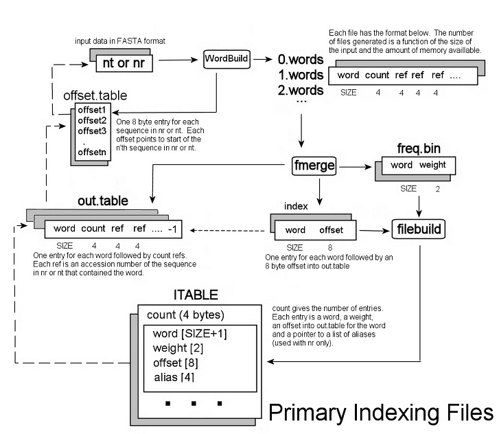
    Flowchart 1
    Source code copies of this code are available at: http://www.cs.uni.edu/~okane/source/
    in the file named idf.src-1.06.tar.gz (note: version number will change with time).

    The IDF weights (freq.bin) Wi for each word i were calculated by:

    Wi= (int) 10 * Log10 ( N / DocFreqi ) (1)

    where N is the total number of sequences, and DocFreq is the total number of sequences in which each word occurred. This weight yields higher values for words whose distribution is more concentrated and lower values for words whose use is more widespread. Thus, words of broad context are weighted lower than words of narrow context.

    For information retrieval, each query sequence was read and decomposed into overlapping 11 character words which were converted to a numeric equivalent for indexing purposes. Entries in a master scoring vector corresponding to data base sequences were incremented by the weight of the word if the word occurred in the sequence and if the weight of the word lay within a specified range. When all words had been processed, entries in the master sequence vector were normalized according to the length of the underlying sequences and to the length of the query. Finally, the master sequence vector was sorted by total weight and the top scoring entries were either displayed with IDF based weights, or scored and ranked by a built-in Smith-Waterman alignment procedure.

    Results

    All tests were conducted on a dual processor Intel Xeon 2.25 mHz system with 4 GB of memory and 5,500 rpm disk drives operating under Mandrake Linux 9.2. Both software systems benefited from the large memory to buffer I/O requests but BLAST, due to the more compact size of its indexing files (about 3 GB vs. 40 GB), was able to load a very substantially larger percentage of its data base into memory which improved its performance in serial trials subsequent to the first.

    Figure 1 shows a graph of aggregate word frequency by weight. The height of each bar reflects the total number of instances of all words of a given weight in the data base. The bulk of the words, as is also the case with natural language text3,7, reside in the middle range.

    
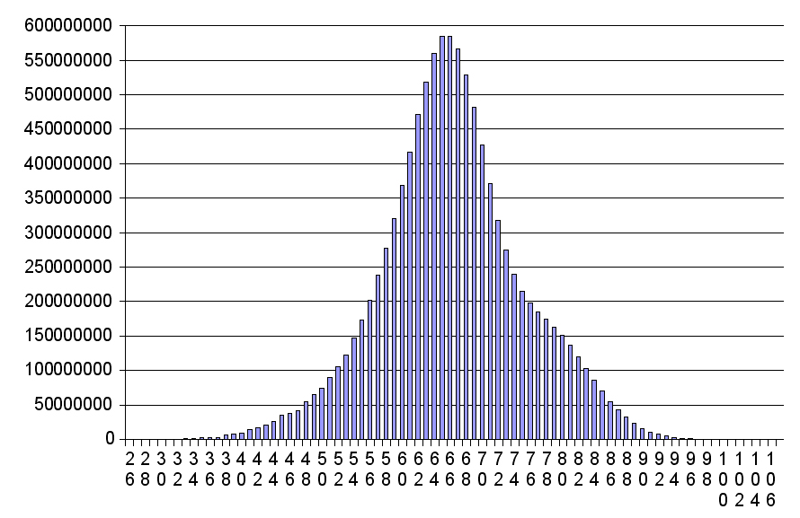
    Figure 1

    Initially, five hundred test queries were randomly generated from the "nt" data base by (1) randomly selecting sequences whose length was between 200 and 800 letters; (2) from each of these, extracting a random contiguous subsequence between 200 and 400 letters; and (3) randomly mutating an average of 1 letter out of 12. While this appears to be a small level of mutation, it is significant for both BLAST and IDF where the basic indexing word size is, by default, 11. A "worst case" of mutation for either approach would be a sequence in which each word were mutated. In our mutation procedure, each letter of a sequence had a 1 in 12 chance of being mutated.

    The test queries were processed and scored by the indexing program with IDF weighting enabled and disabled and also by BLAST. The output of each consisted of 500 sequence title lines ordered by score. The results are summarized in Table 1 and Figures 2 and 3. In Figures 2 and 3, larger bars further to the left indicate better performance (ideally, a single large bar at position 1). The Average Time includes post processing of the results by a Perl program. The Average Rank and Median Rank refer to the average and median positions, respectively, in the output of the sequence from which a query was originally derived. A lower number indicates better performance. The bar at position 60 indicates all ranks 60 and above as well as sequences not found.

    
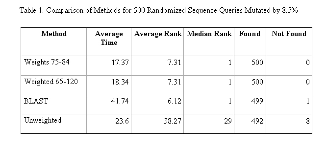
    Table 1
    
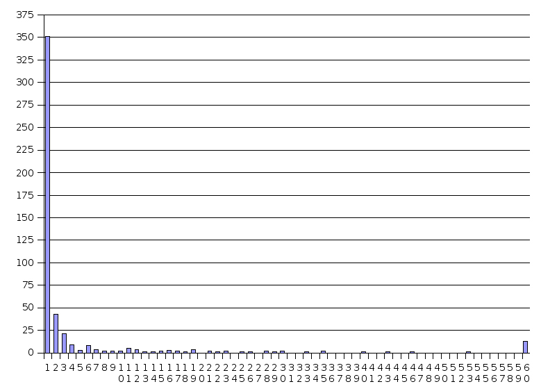
    Figure 2
    
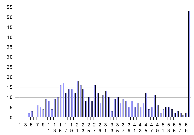
    Figure 3

    When running in unweighted mode, all words in a query were weighted equally and sequences containing those words were scored exclusively on the unweighted cumulative count of the words in common with the query vector. When running in weighted mode, query words were used for indexing if they fell within the range of weights being tested and data base sequences were scored on the sum of the weights of the terms in common with the query vector and normalized for length.

    Figure 3 shows results obtained using the 500 random sequences using indexing only and no weights. The graph in Figure 2 shows significantly better results for the same query sequences with weighted indexing enabled (see also Table 1).

    Subsequently, multiple ranges of weights were tested with the same random sequences. In these tests, only words within certain weight ranges were used. The primary indicators of success were the Average Rank and the number of sequences found and not found. From these results, optimal performance was obtained using weights in the general range of 65 to 120. The range 75 to 84 also yielded similar information retrieval performance with slightly better timing.

    Table 2 shows the results of a series of trials at various levels of mutation and query sequence length. The numbers indicate the percentage of randomly generated and mutated queries of various lengths found. The IDF method is comparable to BLAST at mutations of 20% or less. In all cases, the IDF method was more than twice as fast.

    
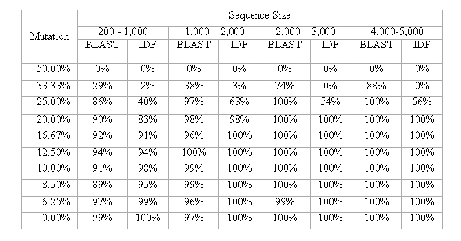
    Table 2

    On larger query sequences (5,000 to 6,000 letters), the IDF weighted method performed slightly better than BLAST. On 25 long sequences randomly generated as noted above, the IDF method correctly ranked the original sequence first 24 times, and once at rank 3. BLAST, on the other hand, ranked the original sequence first 21 times while the remaining 4 were ranked 2, 2, 3 and 4. Average time per query for the IDF method was 47.4 seconds and the average time for BLAST was 122.8 seconds.

    Word sizes other than eleven were tested but with mixed results. Using a word longer than eleven greatly increases the number of words and intermediate file sizes while a smaller value results in too few words relative the number of sequences to provide full resolution.

    A set of random queries was also run against MegaBlast. MegaBlast is a widely used fast search procedure that employs a greedy algorithm and is dependent upon larger word sizes (28 by default). The results of these trials were that the IDF method was able to successfully identify all candidates while MegaBlast failed to identify any candidates. MegaBlast is primarily useful in cases where the candidate sequences are a good match for a target database sequence.

    Figure 4 is a graph of the number of distinct words at each weight in the "nt" data base. The twin peaks were unexpected. The two distinct peaks suggest the possible presence of two .vocabularies. with overlapping bell curves. To test this, we separately indexed the nucleotide data in the NCBI GenBank collections for primates (gbpri*), rodents (gbrod*), bacteria (gbbct*), plants (gbpln*), vertebrates (gbvrt*), invertebrates (gbinv*), patented sequences (gbpat*), viruses (gbvir*), yeast (yeast_gb.fasta) and phages (gbphg*) and constructed similar graphs. The virus, yeast, and phage data bases were too small to give meaningful results and the patents data base covered many species. The other databases, however yielded the graphs shown in Figure 5 which, for legibility, omits vertebrates and invertebrates (see below). In this figure, the composite NT data base graph is seen with the twin peaks as noted from Figure 4. Also seen are the primate and rodent graphs which have similar but more pronounced curves. The curves for bacteria and plants display single peaks. The invertebrate graph is roughly similar to the bacteria and plant graphs and the vertebrate curve is roughly similar to primates and rodents although both these data sets are small and the curves are not well defined.

    
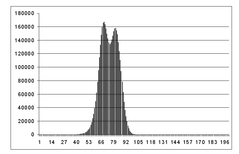
    Figure 4
    
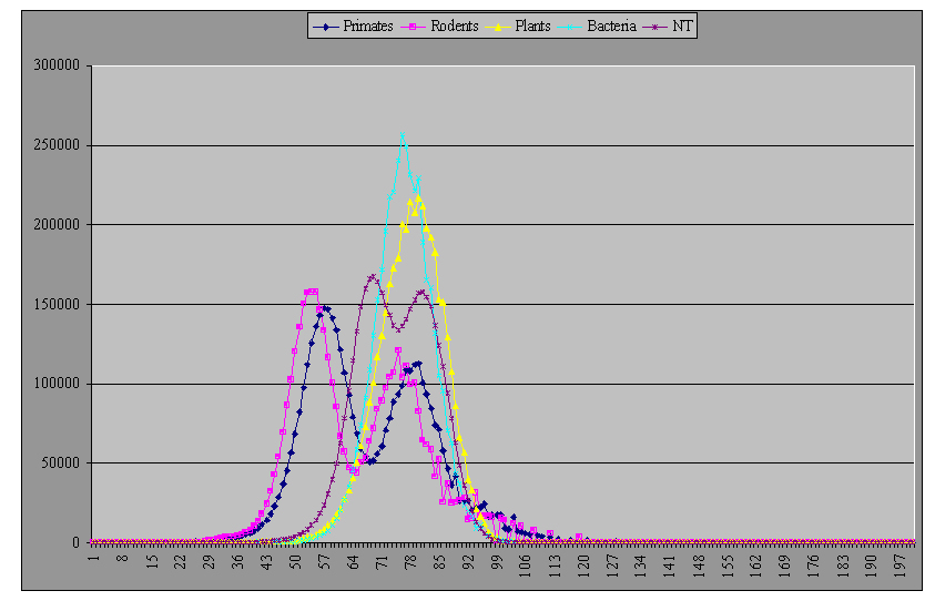
    Figure 5

    The origin and significance of the twin peaks is not fully understood. It was initially hypothesized that it may be due to mitochondrial DNA in the samples. To determine if this were the case, the primate data base was stripped of all sequences whose text description used the term .mitochon*.. This removed 19,647 sequences from the full data bases of 334,537 sequences. The data base was then re-indexed and the curves examined. The curves were unchanged except for a very slight displacement due to a smaller data base (see below). In another experiment, words in a band at each peak in the primate data base were extracted, concatenated, and entered as (very large) queries to the "nt" data base. The resulting sequences retrieved showed some clustering with mouse and primate sequences at words from band 67 to 71 and bacteria more common at band 79 to 83.

    The "nt", primate and rodent graphs, while otherwise similar, are displaced from one another as are the plant and bacteria graphs. These displacements appear mainly to be due to differences in the sizes of the data bases and the consequent effect on the calculation of the logarithmic weights. The NT data base at 12 GB is by far the largest, the primate and rodent data set are 4.2 GB and 2.3GB respectively, while the plant and bacteria databases are somewhat similar at 1.4 GB and 0.97 GB, respectively.

    Conclusions

    The results indicate that it is possible to identify a vocabulary of useful fragment sequences using an n-gram based inverse document frequency weight. Further, an information retrieval system based on this method and incidence scoring is effective in retrieving genomic sequences and is generally better than twice as fast as BLAST and of comparable accuracy when mutations do not exceed 20%. The results also indicate that this procedure works where other speedup methods such as MegaBlast do not.

    Significantly, these results imply that genomic sequences are susceptible to procedures used in natural language indexing and information retrieval. Thus, since IDF or similar weight based systems are often at the root of many natural language information retrieval systems, other more computationally intense text natural language indexing, information retrieval and visualization techniques such as term discrimination, hierarchical sequence clustering, synonym recognition, and vocabulary clustering to name but a few, may also be effective and useful.

45. Miscellaneous Links
    1. Survey of techniques - Developments in Automatic Information Retrieval by G. Salton
       
    2. Origins of language
    3. Irregular English Verbs
    4. Open Directory - Information Retrieval

    Some related lecture slides from UC Berkeley (SIMS 202 Information Organization and Retrieval Instructors: Marti Hearst & Ray Larson)

    1. Introduction to Content Analysis
    2. Introduction to Content Analysis Continued
    3. Term Weighting and Ranking Algorithms
    4. Ranked Retrieval Systems

1. 64 Bit File Addressing.

   For many years, file in C/C++ were addressed using a signed 32 bit pointer. This provided for a file sizes up to 2 GB. However, for many applications, this is inadequate. On newer systems, the file pointer has moved to 64 bits and this provides for effectively unlimited files sizes given currentl levels of disk technology.

   To enable 64 bit file addressing in GNU C/C++, add the following preprocessor commands at the beginning of your program:

   #define _FILE_OFFSET_BITS 64
   #define _LARGE_FILE_SUPPORT
   

   Ordinary functions such as fread(), fwrite(), fopen(), fclose() and so on will work as before. However, the file positioning functions fseek() and ftell() are changed. To randomly reposition a file, declare your file position pointer as type "fpos_t" and use the functions fgetpos() and fsetpos(). For example:

   #define _FILE_OFFSET_BITS 64 #define _LARGE_FILE_SUPPORT #include <stdio.h> #include <stdlib.h> int main() { char buf[128]; FILE *file1; fpos_t fptr; file1=fopen("myfile.dat,"rb+"); // open for read, binary, update (+) if (file1==NULL) { printf("file error\n"); return EXIT_FAILURE; } while (1) { fgetpos(file1,&fptr); // get current file position if (fread(buf,128,1,file1)==0) break; // read a record if ( strncmp(buf,"ABC",3)==0) { // test first 3 chars fsetpos(file1,&fptr); // reposition file buf[0]='a; buf[1]='b'; buf[2]='c'; fwrite(buf,128,1,file1); // re-write record. } } fclose(file1); return EXIT_SUCCESS; }

   Basic Direct Access I/O

   The following takes as input the "translated.txt" file from the Wikipedia data base (it could also be used with the same file from the OSU Medline data base). The program builds two files: one a file of titles from the data base (titles.dat) and the other (index.dat) a set offsets into the first file of the starting byte of each of the titles.

   The program reads each line. For those lines containing the "xxxxx115xxxxx" token indicating a title line, it extracts the title. It finds the current location in "titles.dat" using the "fgetpos()" function. This is the byte offset where the first byte of the title will be written. It writes the title to "titles.dat" and writes the offset of the beginning of the title to "index.dat". The entries in "index.dat" are fixed length (each entry is "sizeof(fpos_t)" bytes. The entries in "titles.dat" are of variable length.

   Note that "titles.dat" is opened with the "wb+" attribute where "w" means write (create), "b" means binary (no CR/LF appended) and "+" means update - that is, the file can be read or written. The file "index.dat" is initially opened for "wb", closed when it is complete, then re-opend for "rb".

   the function "fgetpos()" gets the current byte offset location in a file while the function "fsetpos()" repositions the file to a point specified by the second argument. Note that both functions take the address of the file offset. These functions replace "fseek()" and "ftell()".

   #define _FILE_OFFSET_BITS 64 #define _LARGE_FILE_SUPPORT #include <stdio.h> #include <stdlib.h> #define SIZE 1024 // convert to printable hex char * hex (char *p1, unsigned char * off) { int i; unsigned int j; char h[]="0123456789abcdef"; char *p2=p1; p2=p1; for (i=sizeof(fpos_t)-1; i>=0; i--) { j=*(off+i); *(p1++) = h[(j & 0xf0) >> 4]; *(p1++) = h[j & 0x0f]; } *p1='\0'; return p2; } int main() { char buf[SIZE]; char title[SIZE]; FILE *file1, *file2; fpos_t fptr; file1 = fopen( "titles.dat", "wb+ "); // open for write, binary, update (+) file2 = fopen( "index.dat", "wb" ); // open for write, binary if ( file2 == NULL || file1 == NULL ) { printf("file error\n"); return EXIT_FAILURE; } // read the translated.txt file until EOF (NULL returned). // look for leading xxxxx115xxxxx token, continue if not found. // extract title. get offset in titles.dat file. write title. // write offset to index.dat file. while ( fgets(buf, SIZE, stdin) != NULL ) { if ( strncmp(buf,"xxxxx115xxxxx",13) != 0 ) continue; strcpy( title, &buf[14] ); fgetpos( file1, &fptr ); fputs( title, file1 ); fwrite( &fptr, sizeof(fpos_t), 1, file2); } fclose (file2); file2 = fopen( "index.dat", "rb" ); // open for read, binary // read entry from index.dat, 0 returned when file ends. // position file pointer in titles.dat. // read and print title. while ( fread( &fptr, sizeof(fpos_t), 1, file2) ) { fsetpos( file1, &fptr ); fgets( title, SIZE, file1 ); printf("%s %s", hex( buf, (unsigned char *) &fptr), title); } fclose ( file1 ); fclose ( file2 ); printf("address size=%d\n",sizeof(fpos_t)); return EXIT_SUCCESS; } output: 000000000001addf Flat Earth 000000000001adea Persian language 000000000001adfb Farsi 000000000001ae01 Frances Abington 000000000001ae12 FireWire 000000000001ae1b Finite field 000000000001ae28 Franchising 000000000001ae34 Feynman diagram 000000000001ae44 Food writing 000000000001ae51 Futurama (New York World's Fair) 000000000001ae72 Final Fantasy 3 000000000001ae82 Francesco I Sforza 000000000001ae95 Folk dance 000000000001aea0 Fyodor Dostoevsky 000000000001aeb2 Faith healing 000000000001aec0 Filet Crochet 000000000001aece Furry 000000000001aed4 Fritz Lang 000000000001aedf Food and Drug Administration 000000000001aefc Field extension 000000000001af0c Flood fill 000000000001af17 Francis of Assisi 000000000001af29 Frottage 000000000001af32 First Council of Constantinople 000000000001af52 Fourth Council of Constantinople 000000000001af73 Friedrich Hayek 000000000001af83 Gun 000000000001af87 Fred Reed 000000000001af91 Fred Brooks 000000000001af9d Factoid 000000000001afa5 Figured bass 000000000001afb2 Fashion 000000000001afba Fourier transform 000000000001afcc Fat Man 000000000001afd4 False Claims Act 000000000001afe5 U.S. false claims law 000000000001affb Fantastic Four 000000000001b00a Filtration 000000000001b015 Follies 000000000001b01d Functional grammar 000000000001b030 Fick's law of diffusion 000000000001b048 Far East 000000000001b051 Fawlty Towers 000000000001b05f False friend 000000000001b06c False cognate 000000000001b07a Fall (disambiguation) 000000000001b090 Feudal society 000000000001b09f Fergus McDuck 000000000001b0ad Fundamental analysis 000000000001b0c2 Frasier 000000000001b0ca Fethry Duck

   Huffman Coding

   Huffman Coding is a technique to construct a binary tree with a minum weighted path length. Huffman codes are mainly used in compression as they reorder the tree and are generally unsuitable for information retrieval. The following link describes how to construct Huffman Trees.

   Huffman Codes in Mumps

   #+++++++++++++++++++++++++++++++++++++++++++++++++++++++++++++++++++ #+ #+ Mumps Information Storage and Retrieval Software Library #+ Copyright (C) 2005 by Kevin C. O'Kane #+ #+ Kevin C. O'Kane #+ okane@cs.uni.edu #+ #+ #+ This program is free software; you can redistribute it and/or modify #+ it under the terms of the GNU General Public License as published by #+ the Free Software Foundation; either version 2 of the License, or #+ (at your option) any later version. #+ #+ This program is distributed in the hope that it will be useful, #+ but WITHOUT ANY WARRANTY; without even the implied warranty of #+ MERCHANTABILITY or FITNESS FOR A PARTICULAR PURPOSE. See the #+ GNU General Public License for more details. #+ #+ You should have received a copy of the GNU General Public License #+ along with this program; if not, write to the Free Software #+ Foundation, Inc., 59 Temple Place, Suite 330, Boston, MA 02111-1307 USA #+ #++++++++++++++++++++++++++++++++++++++++++++++++++++++++++++++++++++++ # huff.mps April 10, 2005 ^tree(j) set in=in+1 for x=1:1:in write " " write j,! set k=$p(^a(j),"#",2) if k>0 do ^tree(k) set k=$p(^a(j),"#",3) if k>0 do ^tree(k) quit zmain kill ^a set i=1 for do . read a . if '$test break . if a<0 break . set ^a(i)=a_"#" . write "input ",i," weight=",a,! . set i=i+1 set i=i-1 for do . set c=9999 . set m=0 . set n=0 . for j=1:1:i do .. if +^a(j)=0 continue .. for k=j+1:1:i do ... if +^a(k)=0 continue ... set x=^a(j)+^a(k) ... if x<c set c=x set m=j set n=k . if c=9999 break . set i=i+1 . set ^a(i)=c_"#"_m_"#"_n . set ^a(m)=0_"#"_$p(^a(m),"#",2,99) . set ^a(n)=0_"#"_$p(^a(n),"#",2,99) for k=1:1:i write k," ",^a(k),! set in=1 do ^tree(i) which, when run, produces: huff.cgi < dat input 1 weight=5 input 2 weight=10 input 3 weight=15 input 4 weight=20 input 5 weight=25 input 6 weight=30 input 7 weight=35 input 8 weight=40 input 9 weight=45 input 10 weight=50 1 0# 2 0# 3 0# 4 0# 5 0# 6 0# 7 0# 8 0# 9 0# 10 0# 11 0#1#2 12 0#3#11 13 0#4#5 14 0#6#12 15 0#7#8 16 0#9#13 17 0#10#14 18 0#15#16 19 275#17#18 19 17 10 14 6 12 3 11 1 2 18 15 7 8 16 9 13 4 5 which is: 19 | ------------------------------------------- 17 18 ---------------------- --------------------- 10 14 15 16 ---------- -------- --------- 6 12 7 8 9 13 -------- -------- 3 11 4 5 ------- 1 2

   Optimal Weight Balanced Trees

   Knuth's Discussion: (Knuth 1973)

   See also Mumps program to calculate optimal weight balanced trees

   #include <iostream> #include <stdio.h> #define SIZE 100 using namespace std; struct Node { int id; struct Node * left, * right; }; int W(int q[], int p[], int i, int j) { int k,sum=0; for (k=i; k<=j; k++) sum+=q[k]; for (k=i+1; k<=j; k++) sum+=p[k]; return sum; } void TreeCalc(int p[SIZE], int q[SIZE], int c[SIZE][SIZE], int r[SIZE][SIZE], int span, int nodes) { int x[SIZE]={0}; for (int i=0; i<=nodes-span; i++) { int j=i+span; c[i][j]=W(q,p,i,j); for (int a=0; a < span; a++) { int k=i+a+1; x[a]=c[i][k-1]+c[k][j]; } int m=x[0]; // initial value of minimum int mn=0; // initial index into x for (int n=1; n<span; n++) // check for lower min if (x[n]<m) { m=x[n]; mn=n; } c[i][j]=c[i][j]+m; // add min to calc r[i][j]=i+mn+1; // root associated with min } } struct Node * Add(int i,int j,int r[100][100]) { struct Node * p1; if (i==j) return NULL; p1=new struct Node; p1->id=r[i][j]; printf("Add %d\n",p1->id); p1->left = Add(i,r[i][j]-1,r); p1->right = Add(r[i][j],j,r); return p1; } void tprint(struct Node *p1, int indent) { if (p1==NULL) return; tprint(p1->left,indent+5); for (int i=0; i<indent; i++) printf(" "); printf("%d\n",p1->id); tprint(p1->right,indent+5); } int main() { int q[100]={0},p[100]={0},c[100][100]={0},r[100][100]={0},x[100]={0}; int i,j,k,m,n,mn,nodes; // init a dummy test tree. all q's are 0 p[0]=0; p[1]=2; p[2]=3; p[3]=2; p[4]=4; p[5]=2; p[6]=3; p[7]=2; nodes=7; for (i=1; i<21; i++) printf(" %d",p[i]); printf("\n\n"); // trivial nodes for (i=0; i<=nodes; i++) c[i][i]=0; for (i=1; i<=nodes; i++) TreeCalc(p, q, c, r, i, nodes); // print matrix // horizontal caption printf(" "); for (i=1; i<=nodes; i++) printf("%2d ",i); printf("\n"); printf(" "); for (i=0; i<=nodes; i++) printf("---",i); printf("\n"); // vertical caption and rows for (i=0; i<=nodes; i++) { printf("%2d: ",i); for (j=1; j<=nodes; j++) printf("%2d ",r[i][j]); printf("\n"); } // build the tree useing dummy root node struct Node *root=NULL; // dummy node - tree will be hung from it root=new struct Node; root->left = root->right = NULL; root->left = Add(0,nodes,r); // tree spanning (0,nodes) //print tree tprint(root->left,5); } output: Note: tree prints leftmost node first. To visualize, rotate 90 degrees clockwise then mirror image. 1 2 3 4 5 6 7 ---------------- 0: 1 2 2 2 4 4 4 1: 0 2 2 3 4 4 4 2: 0 0 3 4 4 4 4 3: 0 0 0 4 4 4 6 4: 0 0 0 0 5 6 6 5: 0 0 0 0 0 6 6 6: 0 0 0 0 0 0 7 7: 0 0 0 0 0 0 0 Add 4 Add 2 Add 1 Add 3 Add 6 Add 5 Add 7 1 2 3 4 5 6 7

   Hu-Tucker Weight Balanced Binary Trees

   Hu-Tucker trees are weight balanced binary trees that retain the original alphabetic ordering of their nodes. Calculation of the tree is fast.

   1. Knuth's Discussion: (Knuth 1973)
   2. Another discussion

   Self Adjusting Balanced Binary Trees (AVL)

   Self adjusting balanced binary AVL trees are trees where the distance from the root to each node does not differ by more that +/- 1. The trees are re-balanced after each insertion and deletion. Consequently, they maintain a consistent level of search performance regardless of the order in which the keys are inserted. For a discussions:

   1. AVL Trees
   2. A C++ discussion and implementation

   B-Trees

   B-trees are balanced n-way trees that are very usefile for file structures and widely used in one form or another.

   See also: http://en.wikipedia.org/wiki/B-tree

   // Example b-tree // using ftello(), fseeko(), fread(), fwrite(). // Copyright (c) 2007, 2008 Kevin C. O'Kane /* This program is free software: you can redistribute it and/or modify it under the terms of the GNU General Public License as published by the Free Software Foundation, either version 3 of the License, or (at your option) any later version. This program is distributed in the hope that it will be useful, but WITHOUT ANY WARRANTY; without even the implied warranty of MERCHANTABILITY or FITNESS FOR A PARTICULAR PURPOSE. See the GNU General Public License for more details. You should have received a copy of the GNU General Public License along with this program. If not, see <http://www.gnu.org/licenses/>. */ #define _FILE_OFFSET_BITS 64 #define _LARGE_FILE_SUPPORT #include <stdio.h> #include <stdlib.h> #include <string.h> #include <unistd.h> #include <time.h> // -------------- BTREE PARAMETERS --------------------- // NBR_ITEMS must be even #define NBR_ITEMS 10 #define KEY_SIZE 32 #define FNAME 128 #define BUF_SIZE 128 #define TREE_NAME "btree.dat" // #define PRINT #define STORE 0 #define RETRIEVE 1 #define DELETE 2 #define CLOSE 3 #define TREEPRINT 4 struct entry { char key[KEY_SIZE]; off_t data; }; struct block { struct entry item[NBR_ITEMS+1]; off_t pointer[NBR_ITEMS+2]; }; static struct block tmp2; static struct entry up; static off_t loc1; int add_rec(FILE *, off_t , char *, off_t ); struct entry * search(FILE *,char *, off_t); void dump(char *, FILE *f,off_t root); void dump1(off_t, struct block); struct entry * Btree(int, char *, off_t); void printTree(FILE *bt, off_t root); // -------------- BTREE PARAMETERS --------------------- int MAX,MAX1; int main() { FILE *input; char buf[BUF_SIZE]; char key[KEY_SIZE]; off_t data; char * p1; time_t t1,t2; int i=0; t1=time(NULL); input=fopen("btreedata","r"); while (fgets(buf,BUF_SIZE,input)!=NULL) { // read input file i++; buf[strlen(buf)-1] = '\0'; // chop new line #ifdef PRINT printf("add ------------------------> "); puts(buf); #endif p1=strtok(buf,","); // tokens will be delimited by commas if (p1==NULL || strlen(p1)>KEY_SIZE-1) { printf("Error on input\n"); return EXIT_FAILURE; } strcpy(key,p1); p1=strtok(NULL,","); if (p1==NULL || strlen(p1)>KEY_SIZE-1) { printf("Error on input\n"); return EXIT_FAILURE; } sscanf(p1,"%lld",&data); if (Btree(STORE,key,data) == NULL) return EXIT_FAILURE; } printf("BEGIN RETRIEVE PHASE\n"); rewind(input); // go back to start of input file MAX=MAX1=0; while (fgets(buf,BUF_SIZE,input)!=NULL) { // read input file struct entry *t1; MAX=0; buf[strlen(buf)-1] = '\0'; // chop new line p1=strtok(buf,","); // tokens will be delimited by commas if ( (t1=Btree(RETRIEVE,p1,0)) ==NULL) { printf("not found %s\n",p1); return EXIT_FAILURE; } #ifdef PRINT else printf("%s %lld\n",t1->key,t1->data); #endif if (MAX>MAX1) MAX1=MAX; } Btree(TREEPRINT,NULL,0); printf("Maximum tree depth = %d\n",MAX1); Btree(CLOSE,p1,0); printf("Total time=%d\n",time(NULL)-t1); return EXIT_SUCCESS; } //++++++++++++++++++++++++++++++++++++++++++++++++++++++++++++++++++++++++++++++ struct entry * Btree(int action, char *key, off_t data) { static FILE * btree = NULL; off_t root; if (action == CLOSE) { if ( btree != NULL ) fclose (btree); btree = NULL; return NULL; } if (action == RETRIEVE) { if ( btree == NULL ) return NULL; return search(btree,key,0); } if (btree == NULL ) { // file not open if ( access(TREE_NAME,F_OK) ) { // true if file not found btree=fopen(TREE_NAME,"w+"); // open for create read/write if (btree==NULL) { printf("Error on btree file\n"); return NULL; } root = -1; // has no root block yet /* first 8 bytes of file hold the disk pointer to the root block. */ fwrite(&root,sizeof(off_t),1,btree); // create root record } /* file exists - do not re-create */ else { btree=fopen(TREE_NAME,"r+"); if (btree==NULL) { printf("Error on btree file\n"); return NULL; } } } if (action == TREEPRINT) { fseeko(btree,0,SEEK_SET); // root fread(&root,sizeof(off_t),1,btree); printTree(btree,root); return NULL; } if (action != STORE) return NULL; if (add_rec(btree,0,key,data)) { // 0 means use root /* special case - if add_rec() returns non-zero it means a root split is needed */ off_t root; int j; fseeko(btree,0,SEEK_SET); // old root fread(&root,sizeof(off_t),1,btree); // advances fp for (j=1; j<NBR_ITEMS+1; j++) { // zap it tmp2.pointer[j]=-1; tmp2.item[j].key[0]='\0'; tmp2.item[j].data=-1; } strcpy(tmp2.item[0].key,up.key); // key sent up from below tmp2.item[0].data=up.data; // data sent up from below tmp2.pointer[0]=loc1; // less than child tmp2.pointer[1]=root; // old root block fseeko(btree,0,SEEK_END); // find eof root=ftello(btree); fwrite(&tmp2,sizeof(struct block),1,btree); // write new root fseek(btree,0,SEEK_SET); fwrite(&root,sizeof(off_t),1,btree); // new root } strcpy(up.key,key); up.data=data; return &up; } int add_rec(FILE *f, off_t start, char *key, off_t data) { off_t root,off1,off2,off3; int i,j,k; struct block tmp1; int flg1; loc1=-1; /* if start is zero, we load the address of the root block into root */ if (start==0) { fseeko(f,0,SEEK_SET); // move to beginning of file fread(&root,sizeof(off_t),1,f); // reading advances the fp } else root=start; // begin with a block other than root /* if root is -1, special case - no tree exists yet - make the first (root) block. */ if (root == -1 ) { /* build a block in tmp1 copy key into first slot copy data into first slot make child ptr -1 (points to nothing) */ strcpy(tmp1.item[0].key,key); // key tmp1.item[0].data=data; // data pointer tmp1.pointer[0]=-1; // child /* zero-out the remainder of the block */ for (i=1; i<NBR_ITEMS+1; i++) { // zero the rest tmp1.item[i].key[0]='\0'; tmp1.item[i].data=-1; tmp1.pointer[i]=-1; } tmp1.pointer[NBR_ITEMS+1]=-1; // top end down pointer /* write this record out and put its address in the root address ares (first 8 bytes). */ root=ftello(f); // where are we? fwrite(&tmp1,sizeof(struct block),1,f); // write first block fseek(f,0,SEEK_SET); // move to beginning fwrite(&root,sizeof(off_t),1,f); // new root return 0; // done } /* a tree exists */ fseeko(f,root,SEEK_SET); // move to root address fread(&tmp1,sizeof(struct block),1,f); // read block flg1=0; /* start searching this block */ for (i=0; i<NBR_ITEMS; i++) { if ( strlen(tmp1.item[i].key)==0) { flg1=1; // empty key found - end of keys break; } if ( (j=strcmp(key,tmp1.item[i].key)) == 0 ) { // compare keys tmp1.item[i].data=data; // found - just update data pointer fseeko(f,root,SEEK_SET); fwrite(&tmp1,sizeof(struct block),1,f); return 0; // done } if (j>0) continue; // search key greater than recorded key break; // search key less than recorded key // not in this block } if (tmp1.pointer[i]>=0) { // lower block exists - descend if ( add_rec(f,tmp1.pointer[i],key,data)==0 ) // if not 0, a key was sent up return 0; // finished - no key sent up. strcpy(key,up.key); // a split occurred below and this key was sent up data=up.data; // data pointer sent up } // insert into long block - block has one extra slot for (j=NBR_ITEMS; j>=i; j--) { // shift to create opening tmp1.pointer[j]=tmp1.pointer[j-1]; tmp1.item[j]=tmp1.item[j-1]; } tmp1.pointer[i]=loc1; // child ptr - zero or sent from below strcpy(tmp1.item[i].key,key); // key being added tmp1.item[i].data=data; // data being added for (k=0; k<NBR_ITEMS+1; k++) if (strlen(tmp1.item[k].key)==0) break; // find end of block (k) if (k<NBR_ITEMS) { // easy insert - block had space fseeko(f,root,SEEK_SET); fwrite(&tmp1,sizeof(struct block),1,f); return 0; // block ok } // split block - block full strcpy(up.key,tmp1.item[NBR_ITEMS/2].key); // key to be sent up up.data=tmp1.item[NBR_ITEMS/2].data; // data to be sent up // tmp2 will be the low order block resulting from the split for (j=0; j <= NBR_ITEMS/2; j++) { // copy low order data from tmp1 tmp2.pointer[j]=tmp1.pointer[j]; tmp2.item[j]=tmp1.item[j]; // structure copy } for (j = NBR_ITEMS/2+1; j < NBR_ITEMS+1; j++) { // zap the remainder tmp2.pointer[j]=-1; tmp2.item[j].key[0]='\0'; tmp2.item[j].data=-1; } tmp2.item[NBR_ITEMS/2].key[0]=0; tmp2.item[NBR_ITEMS/2].data=-1; fseeko(f,0,SEEK_END); // advance to endfile and record location loc1=ftello(f); fwrite(&tmp2,sizeof(struct block),1,f); // write low block out // tmp1 is the high order block resulting from the split for (j=0; j<NBR_ITEMS/2; j++) { // shift its contents down to beginning tmp1.pointer[j]=tmp1.pointer[NBR_ITEMS/2+j+1]; tmp1.item[j]=tmp1.item[NBR_ITEMS/2+j+1]; } for (j=NBR_ITEMS/2; j<NBR_ITEMS+1; j++) { // zap its high items tmp1.pointer[j]=-1; tmp1.item[j].key[0]='\0'; tmp1.item[j].data=-1; } tmp1.pointer[NBR_ITEMS/2+1]=tmp1.pointer[NBR_ITEMS+1]; // move its high end child ptr tmp1.pointer[NBR_ITEMS+1]=-1; // zap it tmp1.item[NBR_ITEMS+1],key[0]=0; // zap it fseeko(f,root,SEEK_SET); fwrite(&tmp1,sizeof(struct block),1,f); // write high half return 1; // key/data/child ptr being sent up } struct entry * search(FILE * f, char *key, off_t root) { off_t off1,off2,off3; int i,j; static struct block tmp1; int flg1; MAX++; if (root==0) { fseeko(f,0,SEEK_SET); fread(&root,sizeof(off_t),1,f); // advances fp } fseeko(f,root,SEEK_SET); fread(&tmp1,sizeof(struct block),1,f); flg1=0; for (i=0; i<NBR_ITEMS; i++) { if ( strlen(tmp1.item[i].key)==0) { flg1=1; break; } // empty key if ( (j=strcmp(key,tmp1.item[i].key)) == 0 ) { return &tmp1.item[i]; } if (j>0) continue; break; } if (tmp1.pointer[i]>=0) { // descend - may be high key root=tmp1.pointer[i]; return search(f,key,root); } return NULL; } void dump(char * cap, FILE *f,off_t root) { struct block tmp; int i; fseeko(f,root,SEEK_SET); fread(&tmp,sizeof(struct block),1,f); printf("***dump=%s from block nbr %lld\n",cap,root); for (i=0; i<NBR_ITEMS+1; i++) { printf("%d key=%s %lld %lld\n",i,tmp.item[i].key,tmp.item[i].data,tmp.pointer[i]); } return; } void dump1(off_t r, struct block tmp) { int i; printf("\n***dump from block %lld***\n",r); for (i=0; i<NBR_ITEMS+1; i++) { printf("%d key=%s %lld %lld\n",i,tmp.item[i].key,tmp.item[i].data,tmp.pointer[i]); } return; } void printTree(FILE *bt, off_t root) { int i; struct block tmp1; fseeko(bt,root,SEEK_SET); fread(&tmp1,sizeof(struct block),1,bt); for (i=0; i<NBR_ITEMS; i++) { if ( strlen(tmp1.item[i].key)==0) { // empty key if (tmp1.pointer[i] > 0 ) printTree(bt, tmp1.pointer[i]); return; } if (tmp1.pointer[i] > 0 ) printTree(bt, tmp1.pointer[i]); printf("%s,%lld\n", tmp1.item[i].key, tmp1.item[i].data); } return; }

   Soundex Coding

   Soundex is a technique (patent number 1,261,167 on April 2, 1918) to convert words that sound like one another into common codes. It was originally (and still is) used for telephone directory assistance to permit operators to quickly access the phone numbers based on the sound of a name rather than on a detailed spelling fo the name. It works in most cases but not all. The following links detail how to use it:

   Wikipedia soundex page
   Soundex converter
   Soundex and Geneology

   MD5 - Message Digest Algorithm 5

   MD5 From Wikipedia, the free encyclopedia.
   MD5 Homepage (unofficial)

Running information retrieval applications through Apache on Windows

First, install the Windows version of the Apache webserver. This can be downloaded from http://www.apache.org/dist/httpd/binaries/win32/#released . Find the latest file of the form: http://www.apache.org/dist/httpd/binaries/win32/apache_2.2.3-win32-x86-no_ssl.msi, download it then double click on it (it will initiate the self install procedure).

The default install will place these files in your "Program Files" directory on disk C: and the following discussion assumes that you have a default installation.

First start Apache (see instructions - there will be an Apache icon in your start tray which can be used to start and stop Apache). Test your installation by opening your browser and typing in the IP number 127.0.0.1 (this is the loopback IP number for the machine you are on). You should see a display indicating that the server is working.

Next, enter the Apache cgi-bin directory which should be at:

C:\Program Files\Apache Software Foundation\Apache2.2\cgi-bin

This is where you will place executable programs. Move a copy of the Mumps interpreter here ( mumps.exe) and write a small test cgi script program giving it the name example.cgi (NOTE: do not use <tab>'s at the beginning of lines - use blanks):

Example Apache Mumps Script

#!/Program Files/Apache Software Foundation/Apache2.2/cgi-bin/mumps write "Content-type: text/html ",!! write "<html><body>" write "Hello World<p>" for i=1:1:10 write i,"<br>",! write "</body></html>" halt

The first line tells the web server to run the Mumps interpreter and provides the remainder of the file as program code to the interpreter. You run the above by typing into the URL box:

http://127.0.0.1/cgi-bin/example.cgi

The output of the above looks like:

Center for Intelligent Information Retrieval Publications, University of Massachusetts, http://ciir.cs.umass.edu/publications/