Divisor Increment is a two-player number game. The game board consists of a single number V, the initial value of which is 4. Players take turns increasing V by the value by one of its proper divisors, the numbers in [1..V-1] that divide V evenly.
The proper divisors of 4 are 1 and 2. So, the first player can change V to 5 or 6. If V ever becomes 16, then the player "on move" can increase it to 17, 18, 20, or 24.
The players are given a target number T. The person who advances V past T first is the winner, and the other player must bow to her (or him).
Play five games with opponents of your choice. Take turns going first. Your targets in the four games are:
     17
     25
     50
    100
    243
As always, while you play, try develop a strategy for winning the game. Does going first (or second) ever help -- or hurt?
Now, play four games with opponents of your choice. Take turns choosing who goes first. Your targets for these games are:
      20
      64
     125
    1000
What are your strategies?
Do you have any insights about the game?
Here are some things you may have noticed:
So one winning strategy is:
Actually, we can add any odd divisor to V. Choosing a larger value can speed the game up! Just be careful not to take V too high -- or your opponent can make you pay for your impatience.
So, if V always starts at 4, you always want to go first.
Leave 'Em Different is also a two-player number game. Each game begins with a sequence of integers, m..n, where m < n-2. Players take turns removing one integer from the sequence. After n-m-1 turns, only two integers will remain. If they share no divisors other than 1 -- that is, the numbers are co-prime -- then Player 1 (the player who moved first) wins. Otherwise, Player 2 wins.
For example, suppose a game reaches the list [6, 7, 8]. If the player on the move removes 6 or 8, then the remaining two numbers share no divisors. Player 1 wins the game. If the player on the move removes 7, then the remaining numbers share the divisor 2. Player 2 wins the game.
Play several games with opponents of your choice. Take turns going first. Your game boards are:
    [2..6]
    [5..10]
    [10..20]
    [15..30]
As you play, try to develop a strategy for winning the game, including deciding whether you want to go first or second. A human-usable strategy should use as little space and time as possible. What algorithm might a computer, with more short-term memory and a fast CPU, use?
Now, play several more games with opponents of your choice. But take turns choosing who goes first. Play with these game boards:
    [20..30]
    [51..64]
    [125..135]
What are your strategies?
Do you have any insights about the game?
Here are some things you may have noticed:
Certainly, if a win exists among the last three integers, Player 1 can force it.
Does that give Player 2 an advantage?
The goal of the game is to leave or not leave two co-primes remaining at the end. Knowing some features of co-primes may be useful. What features will help us the most? Simple features that lead to easily-computed invariants can give rise to effective strategies. For example:
If k > 1, then k and k+1 are co-prime.
So, one winning strategy for Player 1 is to try to leave two adjacent numbers on the board at the end. For an odd-length board, Player 1 can remove either end and then view the remaining board as a sequence of pairs of integers. She can preserve this invariant by always removing the 'match' to whichever integer Player 2 removes!
So, the initial board length is odd, a player could choose to go first and use this strategy to force a win.
Are there other strategies available?
If the initial board length is even, then Player 1 does not get the last move and so cannot guarantee the "adjacency invariant" used for odd-length boards. The fact that exactly half of the integers are even and one-third are divisible by 3 gives Player 2 a big advantage. How?
Divisor Increment and Leave 'Em Different are good examples of how reasoning backward from an endgame -- called retrograde analysis in the game world -- can help us to discover simple or otherwise useful invariants. This bears some resemblance to the idea of bottom-up reasoning from Session 2 and ties nicely into our topic for today.
<incomplete-notes>
Consider the problem of computing Fibonacci numbers... [...] If we work top-down, we recompute the same value many times. The algorithm is O(2n) in time.
Alternatives? If we have memory to spare, perhaps we could store the values we have computed. After computing fib(n-1), all we have to do is look up the value for fib(n-2). And that applies all the way down the tree!
Even better: In the future, anytime some asks for fib(k) where k < n, all we have to do is look up the value.
(Check out this cached Fibonacci function in Scheme. Can you do better?)
The technique of caching the results of expensive computations and returning a cached result whenever the function sees a repeated input is called memoization. It is an algorithm-design strategy that relies on remembering past results.
... Memoization is fundamentally top-down. We can use the same idea bottom-up. [...]
</incomplete-notes>
Dynamic programming originated as an optimization technique in applied mathematics. The idea is straightforward: build a solution from the bottom-up by solving each subproblem once and storing its result. Whenever possible, compute a solution by combining the values of two sub-problems that have already been solved.
We sometimes use dynamic programming in a way reminiscent of its roots, as a way to optimize an algorithm. Often, we can greatly improve on a top-down algorithm in a straightforward way by taking advantage of common subproblems and working bottom-up.
We saw our first example of this back in Session 2, in the cool algorithm we wrote for the End Number Game. Today, we'll try it out on a different sort of problem.
(Why do we call this technique "dynamic programming" anyway? Because marketing.)
Suppose that the Cubs and the Tigers are playing in the World Series, a best-of-7 sequence of games. Assume that the chance the Cubs win any given game is p and the chance the Tigers win any given game is 1-p.
We are interested in the function P(i, j), the probability that the Cubs win the series when they need to win i more games and the Tigers need to need to win j more games.
Before the series starts, what are the chances that the Cubs win the series? That is, what is P(4,4)?
Let's break this down into smaller steps. First, write a recurrence relation for P(i, j).
Hint: For i > 0 and j > 0, consider the possibility that the Cubs win the next game and the possibility that the Cubs lose the next game. Then, what are the base cases?
~~~~
Let's consider the recursive case first. The Cubs win the next game with a probability of p. Afterwards, they need to win only i-1 games, while the Tigers still need to win j games. The Cubs lose the next game with a probability of 1-p, after which they still need to win i but the Tigers need to win only j-1 games.
The chance the Cubs win the series is the sum of the probabilities of these two alternatives:
P(i,j) = p⋅P(i-1,j) + (1-p)⋅P(i,j-1)
The base cases are easier than it may seem.
So:
    P(0,j) = 1 for all j > 0
    P(i,0) = 0 for all i > 0
What are we to do with this relation?
Now let's suppose that p = 0.4. What is the probability that the Cubs winning the series?
Let's build a 5x5 table, with rows for 0 ≤ i ≤ 4 and columns for 0 ≤ j ≤ 4. We will fill in the table slot-by-slot using your recurrence relation!
The table:
... some things happen in class ...
The formula for computing each cell is straightforward. We can automate the table-building process for the general case:
    INPUT: p = the probability Team 1 wins any game
           n = number of games in series

    q ← 1 - p
    for j ← 1 to ceiling(n/2) do
        P[0,j] ← 1.0
    for i ← 1 to ceiling(n/2) do
        P[i,0] ← 0.0
        for j ← 1 to ceiling(n/2) do
            P[i,j] ← p * P[i-1,j] + q * P[i,j-1]

    return P[ceiling(n/2), ceiling(n/2)]
... and that, my friends, is dynamic programming!
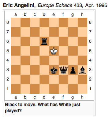
Retrograde Analysis. "Retrograde" problems are a common sort of puzzle in the chess world. If you'd like to try your hand at it, consider this toughie:
There is exactly one possibility. Where did White's king come from, and how? You can find the answer on the Wikipedia page for retrograde analysis.
The Origin of the Name "Dynamic Programming". Richard Bellman created dynamic programming, and he was often asked where the name came from. In a 2002 article in Operations Research, Bellman says:
An interesting question is, "Where did the name, dynamic programming, come from?" The 1950s were not good years for mathematical research. ... I felt I had to do something to shield Wilson and the Air Force from the fact that I was really doing mathematics inside the RAND Corporation [his employer].
He chose "dynamic" because it has positive connotations and is hard to use pejoratively. He chose "programming" as better than "planning" and a positive alternative to mathematics.
Thus, I thought dynamic programming was a good name. It was something not even a Congressman could object to.
One part marketing, one part politics. Ah, the purity of research!