Last time, we played a fun little number game and then saw that there were at least three high-level approaches to designing an algorithm to play it:
Using these techniques in order often works well. A top-down solution is natural and exposes sub-problems, but it sometimes results in solutions that are less efficient than possible or desired. A bottom-up approach can draw on the same sub-problems but combine them in a more efficient way. These two solutions sometimes give us enough experience with the problem to begin to see some relationships that we can use to zoom in and solve the problem more directly.
Keep in mind that an algorithm is a complete, well-defined set of instructions for solving a problem. The input and output of an algorithm must also be defined unambiguously. This means that the sort of instructions we can give a person for doing a task may not be an algorithm.
Okay, that doesn't sound like as much fun as "Let's play a game", but...
The Winter Olympics will be starting in a few weeks. As I watch games such as ice hockey, I sometimes think about how a game score can develop. A team that wins 6-4 might have scored the first six goals of the game and then pulled its starters, or it might have played a tight game that went from 4-4 to 5-4 on a late goal, and then scored a meaningless goal into an open net as time expired.
(Why? The difference might matter to someone trying to determine the relative strengths of all the teams over a set of games. One of the first programs I ever wrote was to assign ratings to a set of competitors based on game results.)
Let's make our thinking more formal.
Two teams play a game of ice hockey. Let's call the teams t1 and t2. The game starts with a score of 0:0 and ends with a score of p1:p2, where t1 and t2 have scored p1 and p2 points, respectively. Given the final game score, we want to compute games(p1:p2), the number of different ways that the score could have been reached.
For example, there is only one way to reach the score 1:0 --
There are three ways to reach 1:2 --
There are ten ways to reach a final score of 3:2. I leave listing them as an exercise for the reader. :-)
Design three algorithms for computing the number of different games:
When you have three algorithms, or feel the need to put one on the back burner, characterize each algorithm's run-time behavior in terms of time and space.
Feel free to work in groups of two or three, if you like. Don't share ideas across groups until I say to.
... lots of fun ensues ....
We can use a divide-and-conquer approach to this problem, much as we did for the End Game last time. Each score p1:p2 can only be reached from two possible scores:
If t1 scores a goal from the first, then we reach our target score. If t2 scores a goal from the second, we also do.
Using this knowledge, we can define a straightforward relationship:
Let's try this out for the game score 1:2...
This definition is inductive, because the function games is defined in terms of itself. The first bullet is the base case, which defines directly answers for two specific problems. The second is the inductive case, which defines the answer to a general problem in terms of one or more simpler cases.
Inductive definitions are a powerful form of shorthand. Though many of you cringe at the idea of an inductive proof, most of you think about certain problems in this way with ease. Reasoning inductively is something humans do automatically, and it turns out to be a useful technique for defining algorithms, too. (Writing a proof requires a few proof-making skills, along with more precision -- and thus more discipline. Just like writing a program.)
Notice, too, that the definition of games is a mathematical function, not a computational function. We may well want to implement it in a program, but for now it defines a set of ordered pairs.
This top-down algorithm works and is quite elegant. But how well does it perform?
Like the top-down algorithm for the End Game, this algorithm recomputes many values of games() multiple times. Look at the next level of that tree...
Does that look familiar? It should. This is a common result for problems that involve combinations of things.
More formally, the algorithm decomposes every score p1:p2 into two sub-problems. Thus, the solution is exponential in the sum p1+p2. This means that the number of recursive calls it makes grows exponentially with changes in p1 and p2.
Can we avoid the recomputations, and thus perhaps some of the exponential load of the algorithm, by eliminating the recursion?
To find games(p1:p2), we need to compute games(n1:n2) for all n1 < p1 and all n2 < p2. But there are only (p1+1) * (p2+1) possible scores! This number doesn't grow exponentially, but multiplicatively. How we can find a solution more quickly?
Let's compute each value once, and remember that result. That is, instead of working from p1:p2 "down to" 0:0, we could work from 0:0 "up to" p1:p2. This is the sort of approach we called dynamic programming last time.
First, let's consider our base case. We know the values for
1:0, 2:0, 3:0, ... p1:0
and
0:1, 0:2, 0:3, ... 0:p2
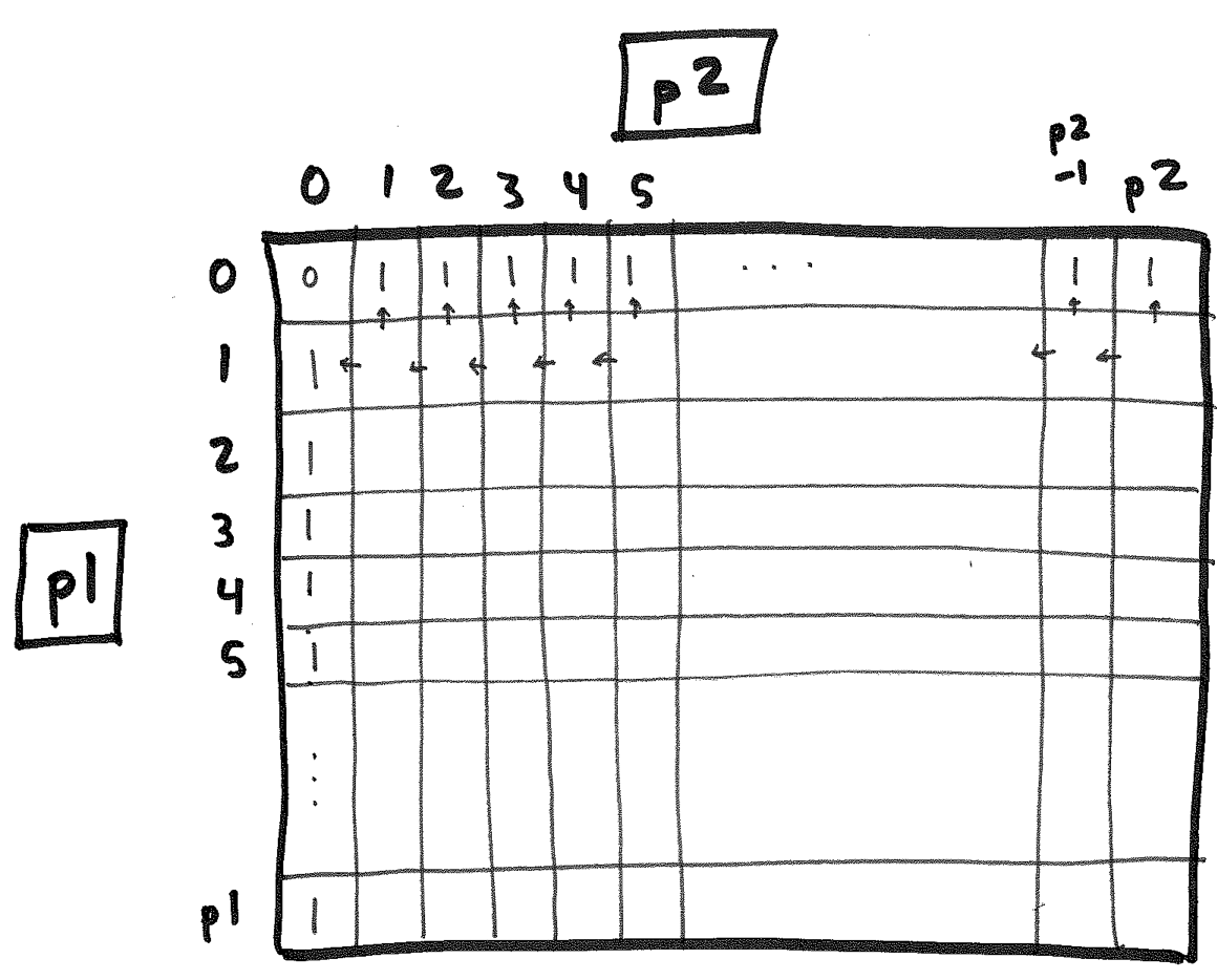
Let's store these values along two of the edges of a (p1+1) * (p2+1) matrix:
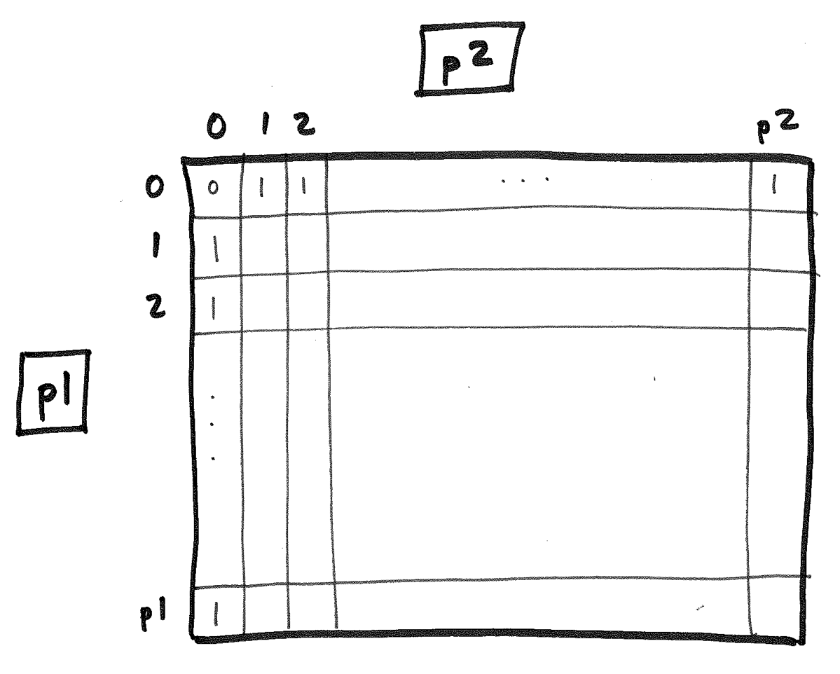
Now, let's consider our inductive case. It applies to every p1 and p2 that are greater than 0. We can fill in the remaining cells of the matrix, one row at a time, using the values in the cells immediately above and to the left!
We fill this in row-by-row and ultimately fill in the entire table:
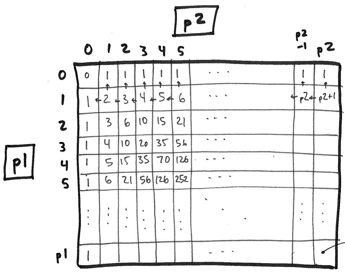
We could speed this process up even further. Notice that games(2:1) = games(1:2). That is, the matrix is symmetric along the 0:0 -p1:p2 diagonal. So we need only compute the values along the diagonal and above, and then copy the corresponding values into the cells below the diagonal.
Even better: If we care only about the final answer, games(p1:p2), we don't even have to remember the whole matrix! Each new entry requires only values from the current row and the preceding row, so we can keep the space of table linear in the larger of p1 and p2.
Wow. We have an algorithm whose time complexity is O( p1⋅p2 ) and whose space complexity is O( max(p1, p2) ). Wow.
Should we be so greedy? If both p1 and p2 are very large, we may have reason to care. Of course, that isn't likely to happen in an ice hockey game, but when computing the number of paths in a computer network it might!
But can we do even better?
On the way from 0:0 to p1:p2, the score increases exactly p1 + p2 times -- once for each goal scored. So, we might view a path from 0:0 to p1:p2 as a (p1+p2)-element sequence of scores where only one of the scores changes between elements. That's how we've been thinking thus far.
Alternatively, though, we could view the game path as a (p1+p2)-element sequence of t1's and t2's, with each item corresponding to which team scored next.
For 1:2, we have three possible sequences:
Aha! Each sequence has exactly p1 t1's and exactly p2 t2s. The different game sequences interleave these values in all possible combinations. So the number of different game paths is simply:
    (p1 + p2)!
    ----------
    p1! X p2!
No recursion. No loop. No table. O(1) space and O( max(p1,p2) ) time to compute the factorials. Now that's zooming in.
It really does help computer scientists to know a little math. You never know when the chance to use it will pop up.
Sometimes, we can find an invariant solution directly. Doing so depends on our background knowledge and our experience with different classes of problems.
Sometimes, it is helpful to work through the approaches in order. Working top-down first and then bottom-up helps you come to understand the problem and its subproblems before trying to create an efficient implementation. Knowledge and understanding usually help us create efficient solutions faster, not slower.
Working top-down and bottom-up often gives us the experience with the problem that we need to find a "zoom-in", direct solution to a new problem.
Exposure, familiarity, experience.
... analyzing the resulting algorithms ...
... best-case, worst-case, average-case ...
Deciding which algorithm to use is often more subtle than it may at first appear. For example, is there a case in which our top-down algorithm for computing games() executes faster than the bottom-up agorithm, or even the zoom-in algorithm? Think about 0:1000...
This also highlights the difference between best-case and average-case. Unfortunately, the average case for the top-down algorithm is also its worst case!