
|
|
A cyclic road contains n gas stations placed at various points along the route. Each station has some number of gallons of gas available. Some stations have more gas than necessary to get to the next station, but other stations do not have enough gas to get to the next station. However, the total amount of gas at the n stations is exactly enough to carry a car around the route exactly once.
Fortunately, our car has a really big tank, so we will always have enough room for whatever gas we find at a station.
Your task: Find a station at which a driver can begin with an empty tank and drive all the way around the road without ever running out of gas.
The input to your algorithm is a list of n integers, one for each station. The ith integer indicates the number of miles a car can travel on the gas available at the ith station.
For simplicity, let's assume that the stations are 10 miles apart. This means that the sum of the n integers will be exactly 10n. We can also assume that we travel clockwise.
The output of your algorithm should be the index of the station at which the driver should begin.
For example, the input might be:
12 6 14 8
If we start at Station 1, we will run out of gas before we get to Station 3, which is twenty miles away. If we start at Station 3, though, we will be able to get back around to Station 3 without running out of gas.
First, you can be assured that this is possible. One of our algorithms will tell us how to do a proof by construction...
Second, some simple attempts fail. For example, we might try finding max(gas[1..n]), and start at that station. This works well for many well-behaved inputs like our example above. But consider this input:
14 1 1 12 12 12 12 12 12 12
If we start at Station 1, we will run out of gas before we reach Station 3! But starting at Station 4 gets us back around just fine.
We could do this in a brute force manner. We could simulate starting at each station and stop as soon as we find a station that never takes the gas tank needle below 0:
    INPUT: gas[1..n]

    for i ← 1 to n do
        tank ← 0
        for j ← i to ((i + n) mod n) do
            tank := tank + gas[j] - 10
            if tank < 0 then next i
        return i
This will solve the problem, if it's solvable. But how efficient is it? That's right: O(n²): for each station, we visit all the stations. We could find a solution on the first pass, but that's not likely.
Is there an invariant that will help us do better? Suppose that we made a "practice run" starting at any station using a car with plenty of extra gas on-board. The amount of gas available on the route is exactly enough to return to the starting station -- so we will end our run with the same amount of fuel we started with!
On the practice run, we watch the gas gauge for its lowest reading, min. This is the extra number of gallons that we carried around with us the whole way.
Call the station at which we observed the lowest reading minStation. We could have started at that station and made the lap, burning our last ounce of extra fuel pulling back into the same station.
So:
    INPUT: gas[1..n]

    minReading ← infinity
    minStation ← -1
    tank ← 0

    for i ← 1 to n do
        if tank < minReading then
           minReading ← tank
           minStation ← i
        tank := tank + gas[i] - 10

    return minStation
How efficient is this approach? That's right: Θ(n). We will alway make exactly one pass!
Like top-down and bottom-up, brute-force is a common design strategy for algorithms, one which we will see throughout the semester. Sometimes we can't do any better, and sometimes it does really well. But usually not. Knowledge almost always helps... Zoom in if you can.
Last time we began to formalize ways to describe and analyze complexity. In order to determine the complexity of an algorithm, we first need to identify the basic operation of the algorithm. (Sometimes, an algorithm has two operations of nearly equal importance, such as comparisons and swaps.) Then we need to count how many times this operation is performed in the course of solving the generic problem.
... iterative algorithms and recursive algorithms offer different challenges...
Last time, we analyzed a simple iterative algorithm for linear search. Today, let's analyze a more complex iterative algorithm, the table-building algorithm for our bottom-up solution to the End Game.
Recall the idea. The game begins with a list L[1..n] of integers. We will build a table with the answers for all possible contiguous sub-lists of L, smallest first, so that making moves is an O(1) look-up.
(This raises the question of batch computing time and distributed computing time. What if we don't have time to do all of the computation up front? Or on a single processor?)
The algorithm:
    for size := 2 to n
        for left := 1 to (n-size+1)
            1. compute and store sum  [left, left+size-1]
            2. compute and store move [left, left+size-1]
            3. compute and store loser[left, left+size-1]
Step 1 is a straightforward O(n) additions in the worst-case, but is O(1) here because we know the answers for smaller lists from previous passes through the loop. We just have to add the new end value! So this costs 1 addition.
Computing the move is done in terms solely of L and previously-computed loser values:
    if size = 2
       then if L[left] > L[left+1]
               then return "left"
               else return "right"
       else if L[left] + loser[left+1, left+size-1] >
                    L[left+size-1] + loser[left, left+size-2]
               then return "left"
               else return "right"
This sub-algorithm requires a comparison and two additions.
Computing the loser sum for a list is done in terms of this iteration's sum and move and the previous iteration's loser values:
    if size = 2
       then return min( L[left], L[left+1] )
       else if move[left, left+size-1] = "left"
               then return sum[left, left+size-1] -
                           (L[left] +
                             loser[left+1, left+size-1])
               else return sum[left, left+size-1] -
                           (L[left+size-1] +
                             loser[left, left+size-2])
This sub-algorithm also requires a comparison and two additions.
This iterative algorithm has three sub-parts! How can we analyze it? The three inner steps are always done together, so we can treat them as a single unit with a total cost of 2 comparisons + 5 additions. Then we count passes through the nested for-loops.
Let's call k = the cost of 2 comparisons + 5 additions. Here is the sum and its reduction: (Click on the image for the full view.)
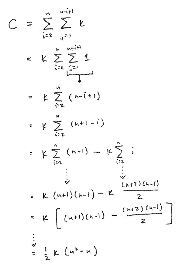
This shouldn't be too surprising. Our intuition leads us to an O(n2) solution. But you want to get some practice doing the analytic arithmetic for cases where you have no intuition, or (worse!) you do have an intuition, but it leads you astray.
Now, let's analyze a recursive algorithm. I would love to analyze our top-down solution to the End Game, too. But move() and loser() are mutually recursive, which would put us in a much deeper hole than we are ready to climb out of just yet. So let's look at more straightforward problem and count the exact number of times its basic operation it performed.
Consider Algorithm Q(n):
    if n = 1
       then return 1
       else return Q(n-1) + n * n * n
Question: What function does Q compute?
Answer: The sum of the first n cubes.
Question: What is the basic operation?
Answer: The multiplication. We could also look at the total cost of 2 multiplications plus 1 addition, and perhaps even the 1 subtraction, but the multiplications tends to dominate.
How many multiplications are done when n=1? 2? 3?
We set up a recurrence relation for the number of multiplications:
    M(1) = 0
    M(n) = M(n-1) + 2
Then, starting with n, we substitute previous values recursively until we find a pattern for n−i:
    M(1)                    = 0
    M(n) =                    M(n-1) + 2
         = (M(n-2) + 2) + 2 = M(n-2) + 4
         = (M(n-3) + 2) + 4 = M(n-3) + 6
         = (M(n-4) + 2) + 6 = M(n-4) + 8
           ...
           ...              = M(n-i) + 2i
Finally, we substitute n−1 for i to reach a solution for the problem of size n:
    M(1)                    = 0
    M(n) =                  = M(n-i) + 2i
           ...
     [substitute i = n-1]   = M(n-(n-1)) + 2(n-1)
                            = M(1) + 2(n-1)
                            =  0   + 2(n-1)
                            = 2(n-1)
So this algorithm performs 2(n-1) multiplications and is O(n).
When analyzing any recursive algorithm, we can use this same process:
Often, the arithmetic for solving a recurrence relation is simpler than that needed to solve the iterative sum.
The Wikipedia pages for these topics are a bit more advanced that we want. Here is a short tutorial on recurrence relations.