Today's game will be quick and simple. Misére Tic-Tac-Toe is played just like the standard children's game. Players take turns placing their mark, usually X or O, in an empty cell of an initially-empty 3x3 grid. The twist... The first player who achieves three in a row loses.
Play this game several times. Take turns going first.
Your task: Can either player force a win? Or force a draw?
What is your strategy?
With optimal play, all games of regular Tic-Tac-Toe end in a tie. The same is true for the Misére version. But can the first player -- seemingly at a disadvantage -- guarantee that she does not lose?
When playing regular Tic-Tac-Toe, there is an enormous advantage to going first and playing in the center. This is especially true as the number of dimensions goes up, for an obvious reason: that square lies on more possible lines of victory than any other square.
So many people begin by thinking that Misére players should avoid the middle square, for a similar reason. It has the most possible "loss lines" running through it, right? But this intuition turns out to be quite wrong. If you avoid the middle square early in the game, then you may be forced into playing their later -- and at that point the many loss lines may already be in place, to your disadvantage.
We can recognize an invariant in the game:
If I always play opposite my opponent's move, then I won't ever be forced to cause a three-in-a-row
-- unless my opponent does it first, in which I will have already won!
So, the drawing strategy for the first player is...
You may recognize this general strategy from many combinatorial games, such as the Prisoner's Dilemma. It runs deep in economic theory and game theory, where it is sometimes called "tit-for-tat" or the "TweedleDum and TweedleDee" theory.
What is the downside of this strategy? The player gives up any chance of winning. That isn't much of a price in the 2-D game, where the second player has trivial ways to draw as well. But as the number of dimensions goes up, the occurrence of a row of three becomes inevitable.
How does this game fit in with our new topic for the week, decrease-and-conquer algorithms?
Let your mind wander back to sixth grade. Multiply 16 by 42 by hand. Then multiply 319 by 111, also by hand. For each problem, write down how many single-digit multiplications you did and how many single-digit additions you did.
("Will this be on the exam?")
Let's consider one last application of divide-and-conquer: multiplying big numbers. How can we improve on the standard solutions to such a straightforward task? As we have begun to see, the conditions in a which a problem is solved can make one approach more or less efficent than others.
Let's start with a little biction. (Hey to CS instructor Mark Jacobson.) Drawing pictures and thinking about them can help us understand anything better, including mathematics.
Consider the value of (x + y)². When many people encounter this for the first time, they assume that (x + y)² = (x²+ y²). If you've had algebra, you know that this is not true. But do you know why? One way to show this is to multiply the expression out, but that requires a fair amount of comfort with algebra.
It also requires a fair amount of work. What if we are lazy?
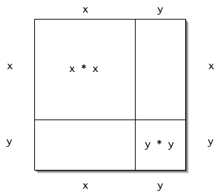
Even a person having little or no experience with algebra can understand this expression if only we draw the right picture:

See, (x + y)² has to be larger than (x²+ y²), because the latter doesn't account for the whole square! What is left over -- two patches of size (xy) -- accounts for the difference, and thus for the correct answer, (x + y)² = (x²+ 2xy + y²).
Drawing a picture like this one will help us to understand how we can use a divide-and-conquer algorithm to multiply large integers.
Why do we even need such an algorithm? Many modern computing applications such as cryptography require the ability to manipulate very large integers, perhaps with hundreds of digits. We can't represent these numbers in single words in hardware and thus not in the primitive types provided by most languages.
As an alternative, we can represent an integer as an array of ints, with the values in lower slots representing the lower-order digits of the number. But how can we do arithmetic on such numbers? The primitive * operator no longer suffices.
What's more, the standard algorithms we know for multiplying numbers are quite inefficient at the machine level. Consider the typical grade-school algorithm for multiplying two n-digit numbers. Each of the n-digits in one is multiplied by each of the n-digits in the other. This means n² multiplications in total. The algorithm also requires 2n-1 additions to tally the resulting columns.
At the machine level, multiplications are generally much more costly than additions. Can we find a way to trade multiplications for additions in a cost-effective way? It would seem impossible to do fewer than n² multiplications, but we can use a divide-and-conquer approach to achieve a remarkable result.
Consider the simple case of 23 * 14. The standard algorithm does four multiplications:
    23 * 14 = (2*10 + 3) * (1*10 + 4)
            = (2*1)*10² + 2*(4*10) + 3*(1*10) + (3*4)
            = (2*1)*10² + (2*4 + 3*1)*10 + (3*4)
               ---         ---   ---        ---
            = 2*10² + 11*10 + 12
            = 322
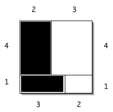
This requires four multiplications. How can we do better? Take a look at this picture, reminiscent of the one above.

Our middle term requires us to compute the areas of the two shaded rectangles. But we already have to compute the areas of the two unshaded rectangles, in order to find the highest- and lowest-order terms. But with a little trick that is easy to see, we only need to do three multiplications:
    (2*4 + 3*1) = [ (2 + 3) * (1 + 4) ] - (2*1) - (3*4)
                    -----------------
This approach works just as well for any two-digit numbers a = a1a0 and b = b1b0. The product c = a*b = c2c1c0 is computed as:
    c2 = a1 * b1
    c0 = a0 * b0

    c1 = (a1+a0)*(b1+b0) - (c2+c0)
Doing two additions instead of one multiplication is a small win, but on a 100- or 1000-digit number, the win accumulates to a huge efficiency gain.
Beautiful.
Try this technique on the two-digit multiplication problem you did earlier, 16 * 42.
This kind of algorithm can be difficult for people to implement. It requires keeping track of extra helper values, and people often find their working memory overloaded. But computers are great at this sort of thing, and the computational advantage can be quite large.
("Yes, this will be on the exam.")
Now for a little traditional divide-and-conquer .
If the number of digits in our numbers, n, is even, we can split a and b right down the middle. Let's denote the split as a = aLaR and b = bLbR. Notice that, arithmetically, this means:
    a = aL10n/2 + aR
    b = bL10n/2 + bR
Now we use our multiplication trick from above to quickly reduce the number of multiplications required:
    c = a * b = (aL10n/2 + aR) * (bL10n/2 + bR)
              = (aL*bL)10n + (aL*bR + aR*bL)10n/2 + (aR*bR)
... where we can replace (aL*bR + aR*bL) with
(aL+aR)*(bL+bR) - (c2+c0)
If n/2 is even, too, we can apply the algorithm again to the parts. If n is a power of two, as it usually is, this algorithm lets decompose the problem recursively until n = 1, where we can do a single multiplications. Of course, we will probably want to stop dividing as soon as the numbers to be multiplied are small enough to fit in memory words. At that point, we can use the machine's primitive multiplication operator.
One last optimization... What if a or b is even? Suppose a is. Then:
c = a * b = (a/2) * (2*b)
As you know from your computer organization course, multiplying and dividing by 2 are the same as shifting the bits of the number left and right, respectively. We don't need to do any multiplications or additions.
Keep doing this until a is odd. This can leave a much simpler problem to be solved, with a shorter a. In the best case, where a is a power of two, we never have to multiply or add. Try it on our old friend 16 * 42. After four shifts, we have 1 * 672, and we are done.
Again: Beautiful.
Let's turn our attention to another way to decompose a problem top-down, decrease-and-conquer. A decrease-and-conquer algorithm follows the same motivation as divide-and-conquer: by solving a smaller problem of the same sort, we can sometimes more easily solve the original problem.
In divide-and-conquer, we typically divide the original problem into two or more subproblems of similar size and solve them all. In decrease-and-conquer, we usually only create one smaller subproblem to solve, by carving off one or two or some small percentage of the input. After solving the subproblem, we incorporate those input values into the solution to the subproblem in order to reach a solution to the original problem.
The simplest case of decrease-and-conquer is decrease-by-one. The typical decrease-by-one algorithm for a problem of size n ...
Even more so than in divide-and-conquer, the 'divide' step is often trivial. In such cases, most of the work goes into the third step, incorporating the lone element into the existing sub-solution.
The prototypical decrease-by-one sorting algorithm is insertion sort. It behaves like a dual of selection sort.
Recall: In selection sort, we go through the remaining elements to select the next element for the sorted subset. Adding the element to the sorted subset is trivial, because it's the next one in line. When we have processed every element, the sorted subset is the answer.
        INPUT: char[0..n-1] line

        for i := 0 to n-1
            minLocation := find slot of smallest element in line[i+1..n-1]
            swap line[minLocation] and line[i]
In insertion sort, though, we take the next element from the next available slot. That's the trivial part. We then insert it into the correct position in the sorted subset. That's where the work happens.
        INPUT: char[0..n-1] line

        for i := 0 to n-1
            insert line[i] into its correct position in line [0..i]
The work of inserting a value into an ordered list [O(n), though with a constant factor of 1/2] is easier than finding a minimal value in an unordered list [a 'hard' O(n)]. So, insertion sort can outperform selection sort on average.
Quick Exercise: How about in the best case? The worst case?
In the best case, an insertion sort's insert step is O(1), giving an overall complexity of O(n). In the worst case, it is hard O(n), resulting in an overall complexity of O(n²).Selection sort is θ(n²) in all cases...
Here is an optimized iterative implementation of the insertion sort:
        for i := 1 to n-1
            v := A[i]
            j := i - 1
            while j ≥ 0 AND A[j] > v
                A[j+1] := A[j]
                j := j - 1
            A[j+1] := v
Quick Exercise: Write a recursive version of insertion sort, where insertion_sort(A) calls insertion(A-1) for some array A-1 that is one smaller than A.
Here is a simple Scheme implementation of a descending insertion sort:
    (define insertion-sort
      (lambda (lon)
        (if (null? lon)
            '()
            (insert-in-order (car lon) (insertion-sort (cdr lon))))))

    (define insert-in-order
      (lambda (n lon)
        (if (null? lon)
            (list n)
            (if (> n (car lon))
                (cons n lon)
                (cons (car lon) (insert-in-order n (cdr lon)))))))
Notice that the general insertion sort algorithm does not commit to how the insertion step is performed. Both the versions above use a *sequential* search for the correct position in the sorted sublist. In the Scheme version, that's natural, as we are working with a linked list. But in the array-based version, we could use a binary search, too.
Quick Exercise: Why not use a binary search?
The short answer is "Binary search is always better, but..." But what? Binary search cuts the number of comparisons from O(n) to O(log n), but we still need to do the same number of swaps [O(n), with a constant factor of 1/2] to make room for the new element. Most implementations of insertion sort do search and swap steps simultaneously, which eliminates the need for a separate search.
Consider the different ways in which the top-down and bottom-up
insertion sorts exemplify "decrease-by-one"... It is in
learning about different ways that an idea can be implemented
-- and in learning how to implement them in different ways --
that you will become a better algorithm designer.